断层中应变场检测方案(粒子图像测速)

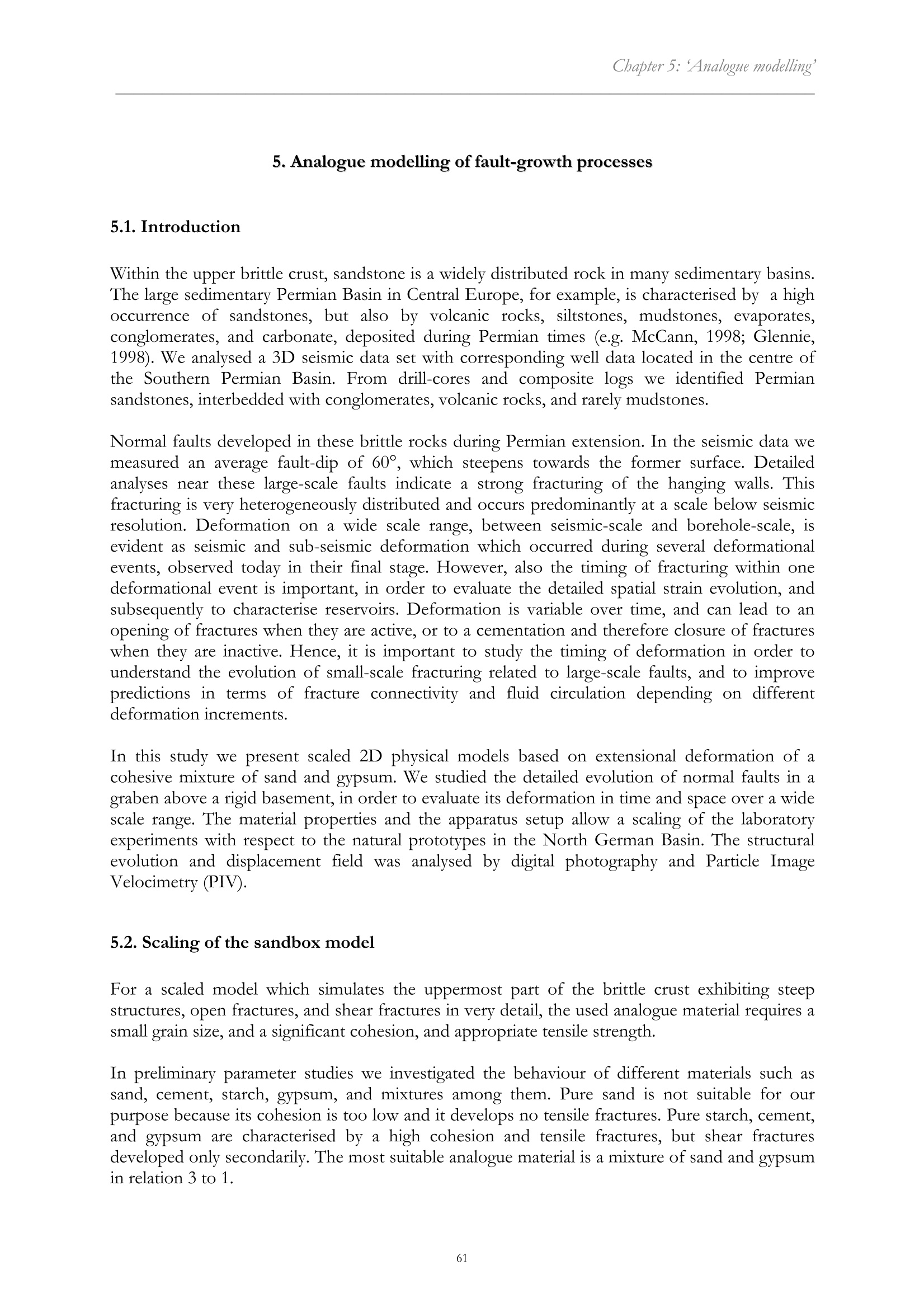
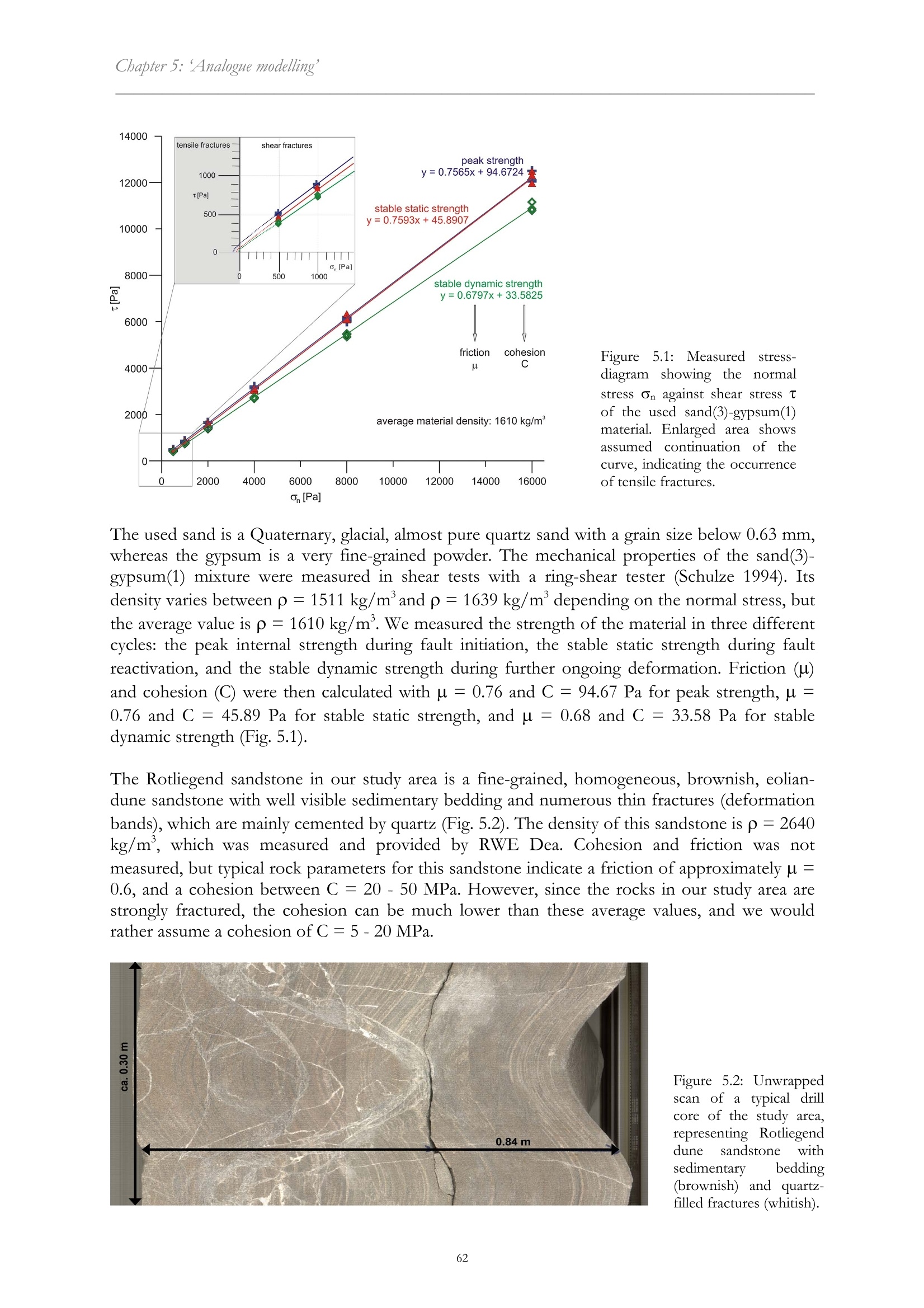
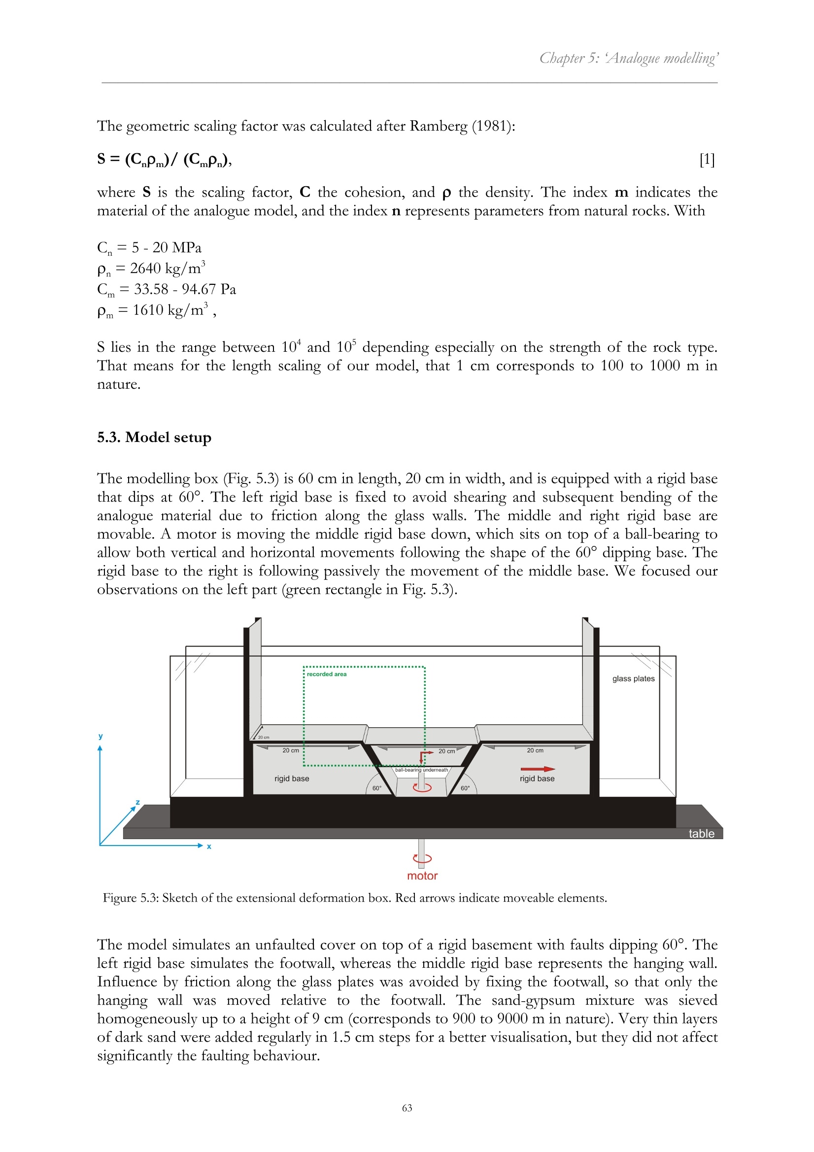
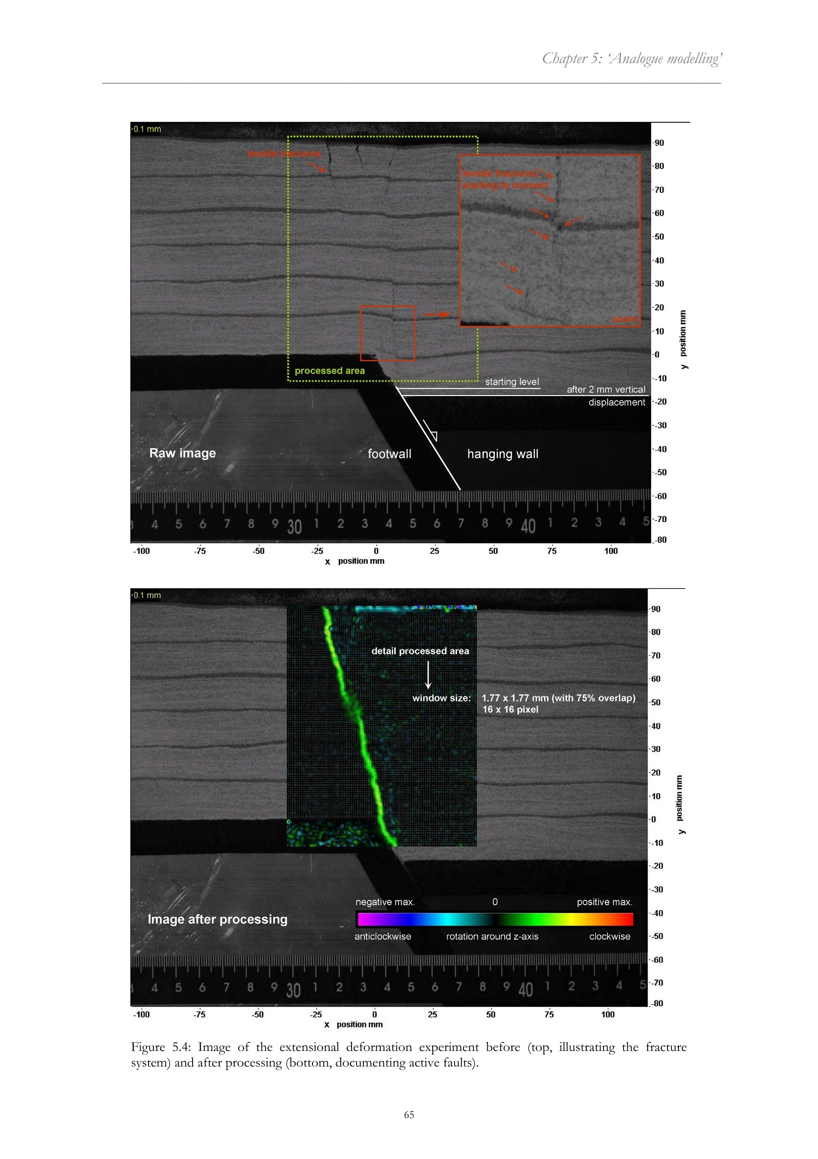
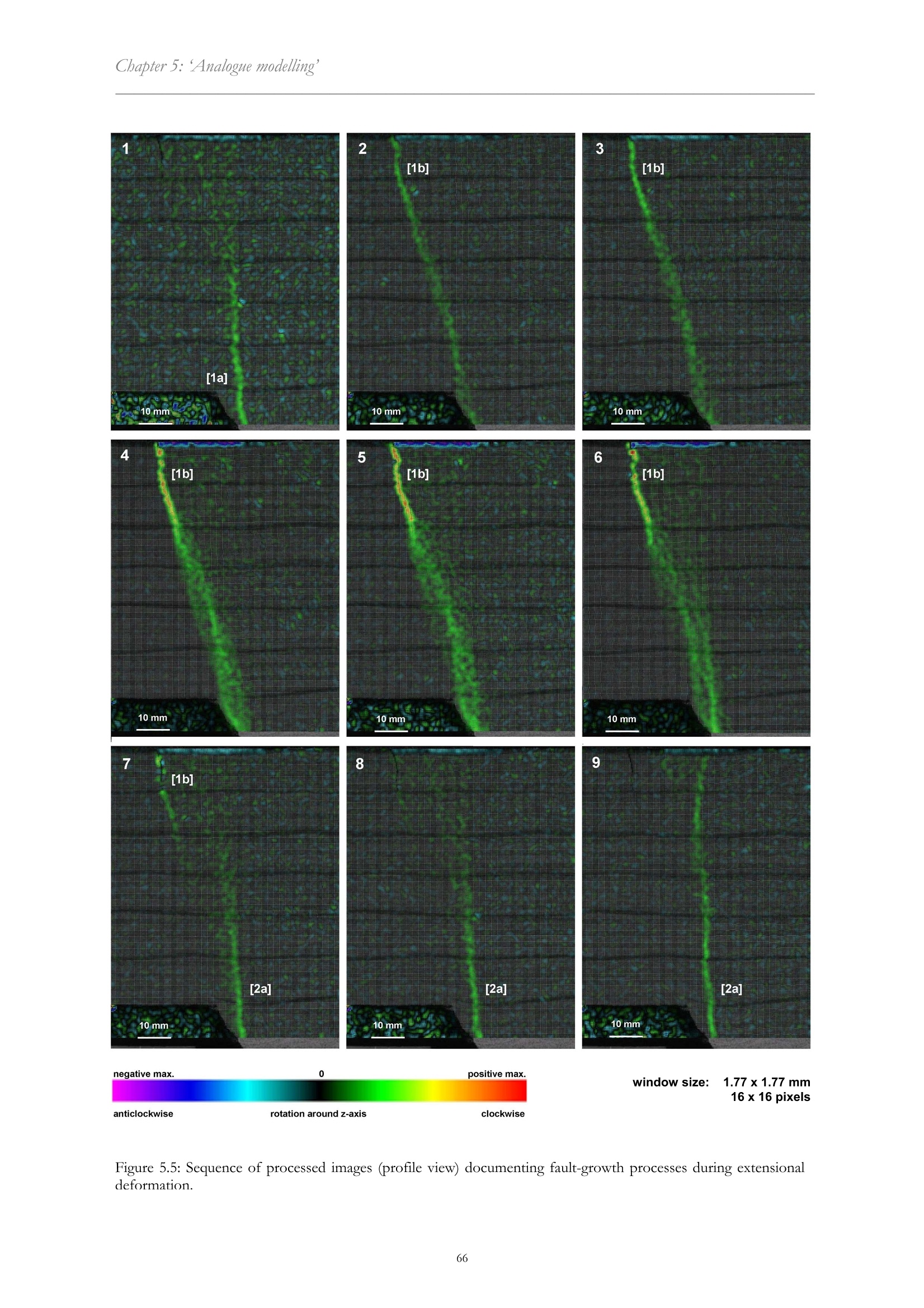
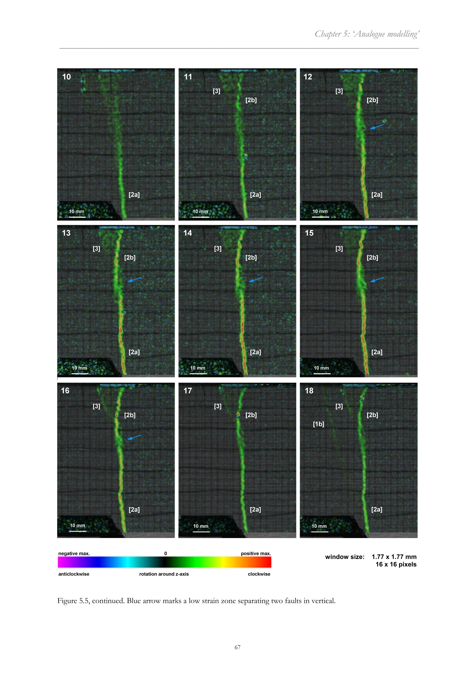
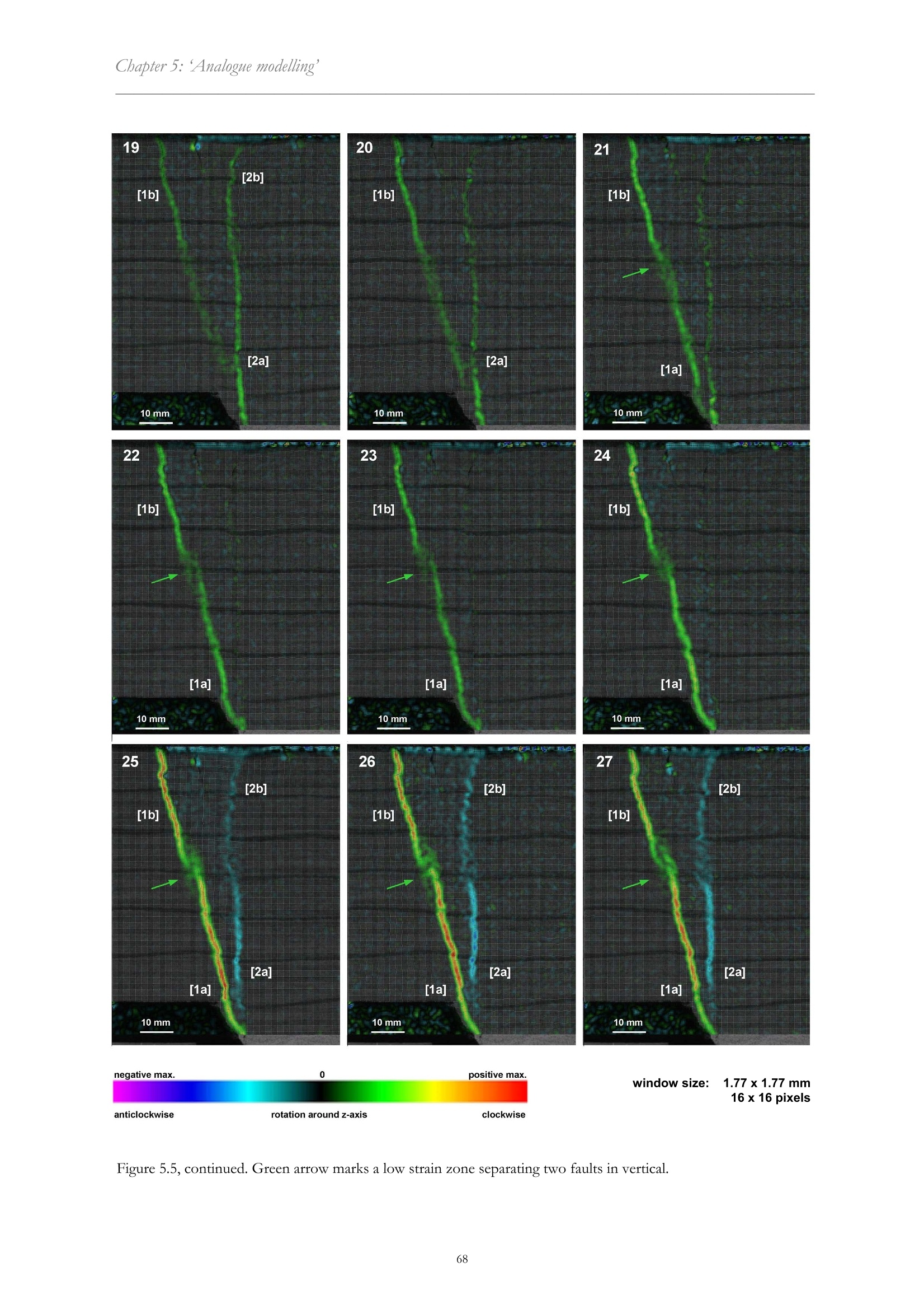
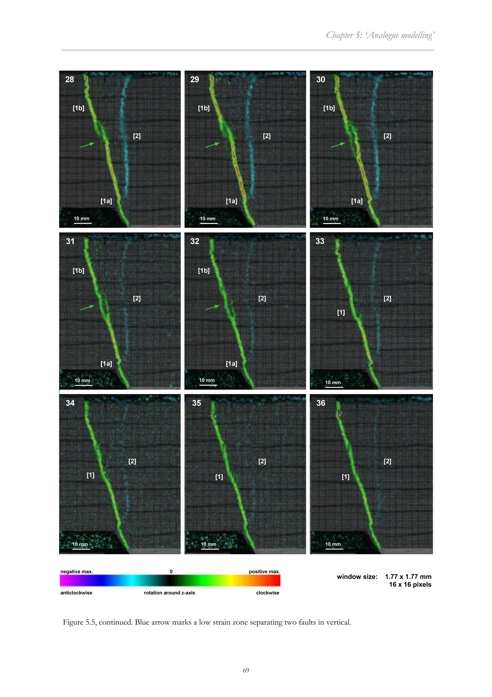
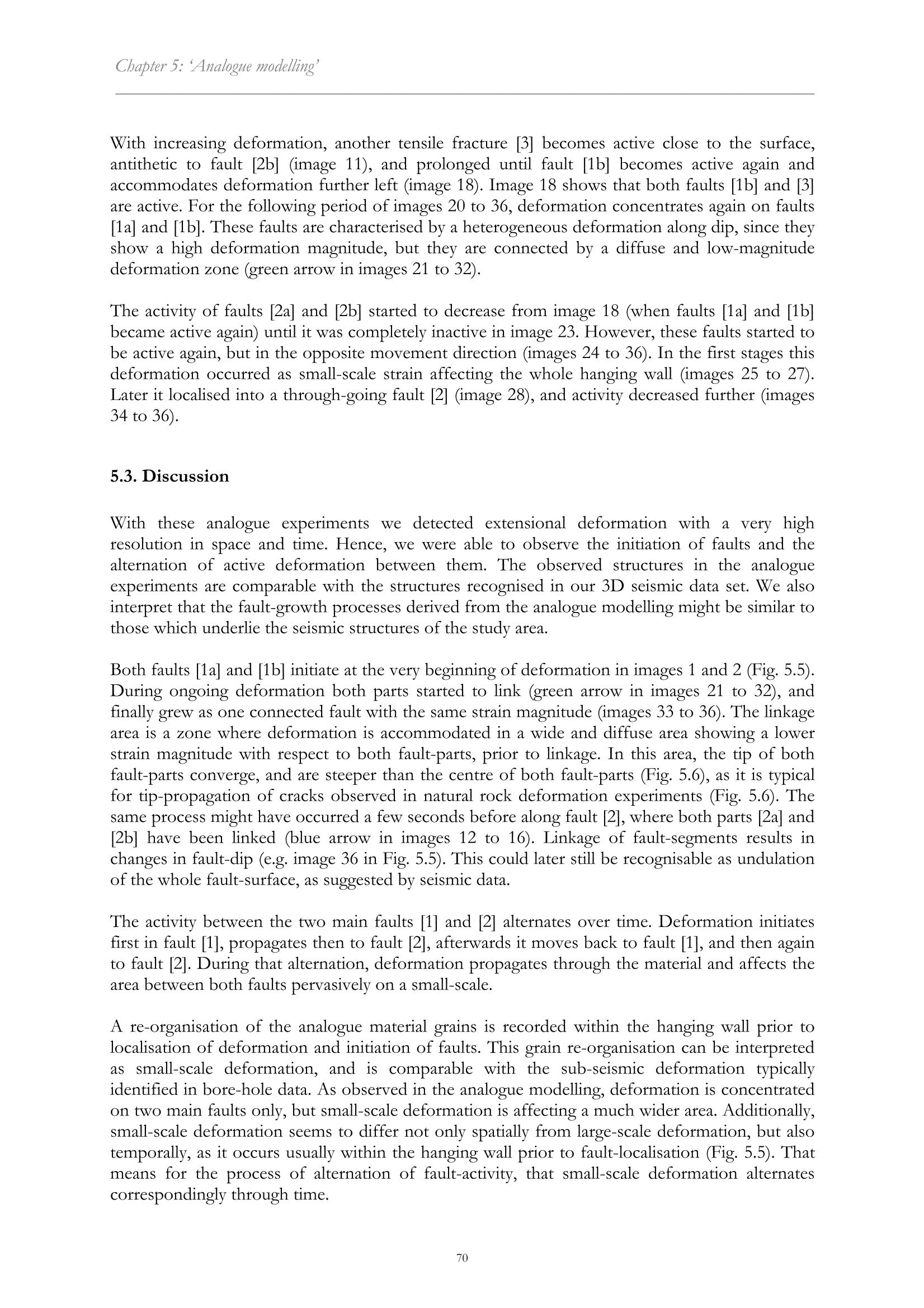
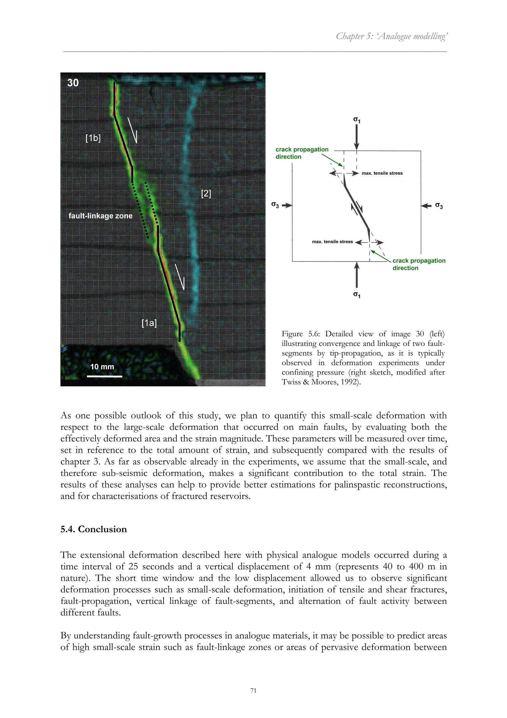
Chapter 5：‘Analogue modelling' 5. Analogue modelling of fault-growth processes 5.1. Introduction Within the upper brittle crust， sandstone is a widely distributed rock in many sedimentary basins.The large sedimentary Permian Basin in Central Europe， for example， is characterised by a highoccurrence of sandstones， but also by volcanic rocks， siltstones， mudstones， evaporates，conglomerates， and carbonate， deposited during Permian times (e.g. McCann， 1998； Glennie，1998). We analysed a 3D seismic data set with corresponding well data located in the centre ofthe Southern Permian Basin. From drill-cores and composite logs we identified Permiansandstones， interbedded with conglomerates， volcanic rocks， and rarely mudstones. Normal faults developed in these brittle rocks during Permian extension. In the seismic data wemeasured an average fault-dip of 60°， which steepens towards the former surface. Detailedanalyses near these large-scale faults indicate a strong fracturing of the hanging walls. Thisfracturing is very heterogeneously distributed and occurs predominantly at a scale below seismicresolution. Deformation on a wide scale range， between seismic-scale and borehole-scale， isevident as seismic and sub-seismic deformation which occurred during several deformationalevents， observed today in their final stage. However， also the timing of fracturing within onedeformational event is important， in order to evaluate the detailed spatial strain evolution， andsubsequently to characterise reservoirs. Deformation is variable over time， and can lead to anopening of fractures when they are active， or to a cementation and therefore closure of fractureswhen they are inactive. Hence， it is important to study the timing of deformation in order tounderstand the evolution of small-scale fracturing related to large-scale faults， and to improvepredictions in terms of fracture connectivity and fluid circulation depending on differentdeformation increments. In this study we present scaled 2D physical models based on extensional deformation of acohesive mixture of sand and gypsum. We studied the detailed evolution of normal faults in agraben above a rigid basement， in order to evaluate its deformation in time and space over a widescale range. The material properties and the apparatus setup allow a scaling of the laboratoryexperiments with respect to the natural prototypes in the North German Basin. The structuralevolution and displacement field was analysed by digital photography and Particle ImageVelocimetry (PIV). 5.2. Scaling of the sandbox model For a scaled model which simulates the uppermost part of the brittle crust exhibiting steepstructures， open fractures， and shear fractures in very detail， the used analogue material requires asmall grain size， and a significant cohesion， and appropriate tensile strength. In preliminary parameter studies we investigated the behaviour of different materials such assand， cement， starch， gypsum， and mixtures among them. Pure sand is not suitable for ourpurpose because its cohesion is too low and it develops no tensile fractures. Pure starch， cement，and gypsum are characterised by a high cohesion and tensile fractures， but shear fracturesdeveloped only secondarily. The most suitable analogue material is a mixture of sand and gypsumin relation 3 to 1. Figure 5.1：：Measured stresS-diagram showing the normalstress On against shear stress Tof the used sand(3)-gypsum(1)material. Enlarged area showsassumed continuation ofthecurve， indicating the occurrenceof tensile fractures. The used sand is a Quaternary， glacial， almost pure quartz sand with a grain size below 0.63 mm，whereas the gypsum is a very fine-grained powder. The mechanical properties of the sand(3)-gypsum(1) mixture were measured in shear tests with a ring-shear tester (Schulze 1994). Itsdensity varies between p =1511 kg/m'andp = 1639 kg/m'depending on the normal stress， butthe average value is p = 1610 kg/m. We measured the strength of the material in three differentcycles： the peak internal strength during fault initiation， the stable static strength during faultreactivation， and the stable dynamic strength during further ongoing deformation. Friction (u)and cohesion (C) were then calculated with p=0.76 and C = 94.67 Pa for peak strength， p=0.76 and C = 45.89 Pa for stable static strength， and u =0.68 and C = 33.58 Pa for stabledynamic strength (Fig.5.1). The Rotliegend sandstone in our study area is a fine-grained， homogeneous， brownish， eolian-dune sandstone with well visible sedimentary bedding and numerous thin fractures (deformationbands)， which are mainly cemented by quartz (Fig. 5.2). The density of this sandstone is p = 2640kg/m’， which was measured and provided by RWE Dea. Cohesion and friction was notmeasured， but typical rock parameters for this sandstone indicate a friction of approximately p=0.6， and a cohesion between C = 20 - 50 MPa. However，since the rocks in our study area arestrongly fractured， the cohesion can be much lower than these average values， and we wouldrather assume a cohesion of C =5-20 MPa. Figure 5.2： Unwrappedscan of a typical drillcore of the study area，representing Rotliegenddune sandstone withsedimentary bedding(brownish) and quartz-filled fractures (whitish). The geometric scaling factor was calculated after Ramberg (1981)： where S is the scaling factor， C the cohesion， and p the density. The index m indicates thematerial of the analogue model， and the index n represents parameters from natural rocks. With p.=2640 kg/m’ Cm=33.58 -94.67 Pa Pm=1610 kg/m’， S lies in the range between 10 and 10'depending especially on the strength of the rock type.That means for the length scaling of our model， that 1 cm corresponds to 100 to 1000 m innature. 5.3. Model setup The modelling box (Fig. 5.3) is 60 cm in length， 20 cm in width， and is equipped with a rigid basethat dips at 60°. The left rigid base is fixed to avoid shearing and subsequent bending of theanalogue material due to friction along the glass walls. The middle and right rigid base aremovable. A motor is moving the middle rigid base down， which sits on top of a ball-bearing toallow both vertical and horizontal movements following the shape of the 60° dipping base. Therigid base to the right is following passively the movement of the middle base. We focused ourobservations on the left part (green rectangle in Fig. 5.3). Figure 5.3： Sketch of the extensional deformation box. Red arrows indicate moveable elements. The model simulates an unfaulted cover on top of a rigid basement with faults dipping 60°. Theleft rigid base simulates the footwall， whereas the middle rigid base represents the hanging wall.Influence by friction along the glass plates was avoided by fixing the footwall， so that only thehanging wall was moved relative to the footwall. The sand-gypsum mixture was sievedhomogeneously up to a height of 9 cm (corresponds to 900 to 9000 m in nature). Very thin layersof dark sand were added regularly in 1.5 cm steps for a better visualisation， but they did not affectsignificantly the faulting behaviour. The experiments were monitored and analysed with a high-resolution digital camera andcorresponding PIV technology (Particle Image Velocimetry). PIV is an optical technique toobserve movements and flows by calculating the displacement field of grains， and allows thecalculation of strain and rotation within the material. During the experiment a sequence ofimages was recorded， and the LAVISION software DaVis calculates the 2D vector field bycomparing the pattern of grains of neighbouring images. Seven experiments have been done with the same experimental setup and material parameters forstatistically relevant repetitions. All experiments have been performed with a final verticaldisplacement of ca. 2.5 cm， during which ca. 630 images have been taken. We carried out the experiment with the following parameters： Optical resolution： 9 pixel/mm (2000 x 2000 pixels for the recorded area) → Resolvable scale： 1 mm to 9 cm (corresponds to 10 m to 9000 m in nature)Vertical displacement rate： 0.16 mm/sOne camera， recording time： 4 pictures/s→ 1 picture every 0.04 mm vertical displacement The low velocity， the high sampling rate， and the high optical resolution allowed a high spatialand temporal resolution during deformation of the analogue material. 5.3.Results All experiments are reproducible since they show similar structural elements and evolution. Theresults of the processed experiment shown here comprise only the very beginning ofdeformation， as it is that part where fault-growth processes were initialised. Therefore， the area ofthe deformation experiment which has been recorded is much larger than the one which hasbeen finally processed with the PIV technology for this purpose (Fig. 5.4). At the beginning of deformation， we observed vertical fractures in the upper part of the material，which open perpendicularly to the surface (tensile fractures). The lower part of the material ischaracterised by very small and short-living tensile fractures oblique to the surface， whichconnect rapidly to build shear fractures (zoomed area of Fig. 5.4). In the processed image， thecolour-code illustrates the rotational strain， in particular the rotation of particles around the z-axis， and indicates a clockwise rotation (synthetic faulting) with green， yellow， and red colours，and an anticlockwise rotation (antithetic faulting) with blue and purple colours， depending on therelative magnitude of rotation. Zero rotation (inactive areas) is shown in black. Several processed images are shown in Figure 5.5， which comprises 36 stages extracted from theinitial deformation part of one representative experiment. Here， only every third image is shown，but also the images in between have been analysed. As it is documented in image 1 of Figure 5.5，the PIV technology also allows measuring the initial re-organisation of grains as small-scaledeformation prior to failure. In image 1， the whole area is affected by subtle deformation， butdeformation localises first in the lower part (fault [1a]). Afterwards， deformation is focused in theupper part (fault [1b])， whereas deformation in the lower part becomes more and more diffuse(images 2 to 5)， propagates towards to right (images 4 to 7)， and localises as vertical fault [2a]growing upwards (images 7 to 12). The previous initiated faults [1a] and [1b] are now inactive，and the vertical faults [2a] and [2b] are active (image 12). Both faults [2a] and [2b] show a higherstrain magnitude than the part in between them (blue arrow in images 12 to 16). 0.1 mm c x position mm Figure 5.4： Image of the extensional deformation experiment before (top， illustrating the fracturesystem) and after processing (bottom， documenting active faults). 10 mm511b]10mm8 9 2al10 mm 2a] 10mm negative max. 0 positive max. window size： 1.77 x 1.77 mm 16x16 pixels anticlockwise rotation around z-axis clockwise Figure 5.5： Sequence of processed images (profile view) documenting fault-growth processes during extensionaldeformation. [3] 2b1 [2a] 16 [3] [2b] [2a] 2a] 10 mm 10mm negative max. 0 positive max. window size： 1.77 x 1.77 mm 16x16 pixels anticlockwise rotation around z-axis clockwise Figure 5.5， continued. Blue arrow marks a low strain zone separating two faults in vertical. 25 27 [2b] 2b] [1b] [16] [2a] 2a] 2a [1a] [1a] 1al 10 mm 10 mm 10 mm negative max. 0 positive max. window size： 1.77 x1.77 mm 16 x 16 pixels anticlockwise rotation around z-axis clockwise Figure 5.5， continued. Green arrow marks a low strain zone separating two faults in vertical. 36 [2] [1] 10 mm negative max. 0 positive max. window size： 1.77 x 1.77 mm 16x 16 pixels anticlockwise rotation around z-axis clockwise With increasing deformation， another tensile fracture [3] becomes active close to the surface，antithetic to fault [2b] (image 11)， and prolonged until fault [1b] becomes active again andaccommodates deformation further left (image 18). Image 18 shows that both faults [1b] and [3]are active. For the following period of images 20 to 36， deformation concentrates again on faults[1a] and [1b]. These faults are characterised by a heterogeneous deformation along dip， since theyshow a high deformation magnitude， but they are connected by a diffuse and low-magnitudedeformation zone (green arrow in images 21 to 32). The activity of faults [2a] and [2b] started to decrease from image 18 (when faults [1a] and [1b]became active again) until it was completely inactive in image 23. However， these faults started tobe active again， but in the opposite movement direction (images 24 to 36). In the first stages thisdeformation occurred as small-scale strain affecting the whole hanging wall (images 25 to 27).Later it localised into a through-going fault [2] (image 28)， and activity decreased further (images34 to 36). 5.3. Discussion With these analogue experimentswe detected extensional deformation with a very highresolution in space and time. Hence， we were able to observe the initiation of faults and thealternation of active deformation between them. The observed structures in the analogueexperiments are comparable with the structures recognised in our 3D seismic data set. We alsointerpret that the fault-growth processes derived from the analogue modelling might be similar tothose which underlie the seismic structures of the study area. Both faults [1a] and [1b] initiate at the very beginning of deformation in images 1 and 2 (Fig. 5.5).During ongoing deformation both parts started to link (green arrow in images 21 to 32)， andfinally grew as one connected fault with the same strain magnitude (images 33 to 36). The linkagearea is a zone where deformation is accommodated in a wide and diffuse area showing a lowerstrain magnitude with respect to both fault-parts， prior to linkage. In this area， the tip of bothfault-parts converge， and are steeper than the centre of both fault-parts (Fig. 5.6)， as it is typicalfor tip-propagation of cracks observed in natural rock deformation experiments (Fig. 5.6). Thesame process might have occurred a few seconds before along fault [2]， where both parts [2a] and[2b] have been linked (blue arrow in images 12 to 16). Linkage of fault-segments results inchanges in fault-dip (e.g. image 36 in Fig. 5.5). This could later still be recognisable as undulationof the whole fault-surface， as suggested by seismic data. The activity between the two main faults [1] and [2] alternates over time. Deformation initiatesfirst in fault [1]， propagates then to fault [2]， afterwards it moves back to fault [1]， and then againto fault [2]. During that alternation， deformation propagates through the material and affects thearea between both faults pervasively on a small-scale. A re-organisation of the analogue material grains is recorded within the hanging wall prior toandilocalisation of deformation and initiation of faults. This grain re-organisation can be interpretedassmall-scale deformation， and is comparable with the sub-seismic deformation typicallyidentified in bore-hole data. As observed in the analogue modelling， deformation is concentratedon two main faults only， but small-scale deformation is affecting a much wider area. Additionally，small-scale deformation seems to differ not only spatially from large-scale deformation， but alsotemporally， as it occurs usually within the hanging wall prior to fault-localisation (Fig. 5.5). Thatmeans for the process of alternation of fault-activity， that small-scale deformation alternatescorrespondingly through time. Figure 5.6： Detailed view of image 30 (left) illustrating convergence and linkage of two fault- segments by tip-propagation， as it is typically observedincdeformation experiments under confining pressure (right sketch， modified after Twiss & Moores， 1992). As one possible outlook of this study， we plan to quantify this small-scale deformation withrespect to the large-scale deformation that occurred on main faults， by evaluating both theeffectively deformed area and the strain magnitude. These parameters will be measured over time，set in reference to the total amount of strain， and subsequently compared with the results ofchapter 3. As far as observable already in the experiments， we assume that the small-scale， andtherefore sub-seismic deformation， makes a significant contribution to the total strain. Theresults of these analyses can help to provide better estimations for palinspastic reconstructions，and for characterisations of fractured reservoirs. 5.4. Conclusion The extensional deformation described here with physical analogue models occurred during atime interval of 25 seconds and a vertical displacement of 4 mm (represents 40 to 400 m innature). The short time window and the low displacement allowed us to observe significantdeformation processes such as small-scale deformation， initiation of tensile and shear fractures，fault-propagation， vertical linkage of fault-segments， and alternation of fault activity betweendifferent faults. By understanding fault-growth processes in analogue materials， it may be possible to predict areasof high small-scale strain such as fault-linkage zones or areas of pervasive deformation between large faults within the model. This can then be compared with the natural example and can helpto estimate the sub-surface fracture density.