


方案详情
文
The following chapter presents the basics of ellipsometry and discusses some recent advances. The article covers the formalism and theory used for data analysis as well as instrumentation. The treatment is also designed to familiarize newcomers to this ßeld.
The experimental focus is on adsorption layers at the air-water and oil-water interface.
Selected examples are discussed to illustrate the potential as well as the limits of this technique. The authors hope, that this article contributes to a wider use of this technique in the colloidal physics and chemistry community. Many problems in our ßeld of science
can be tackled with this technique.
方案详情

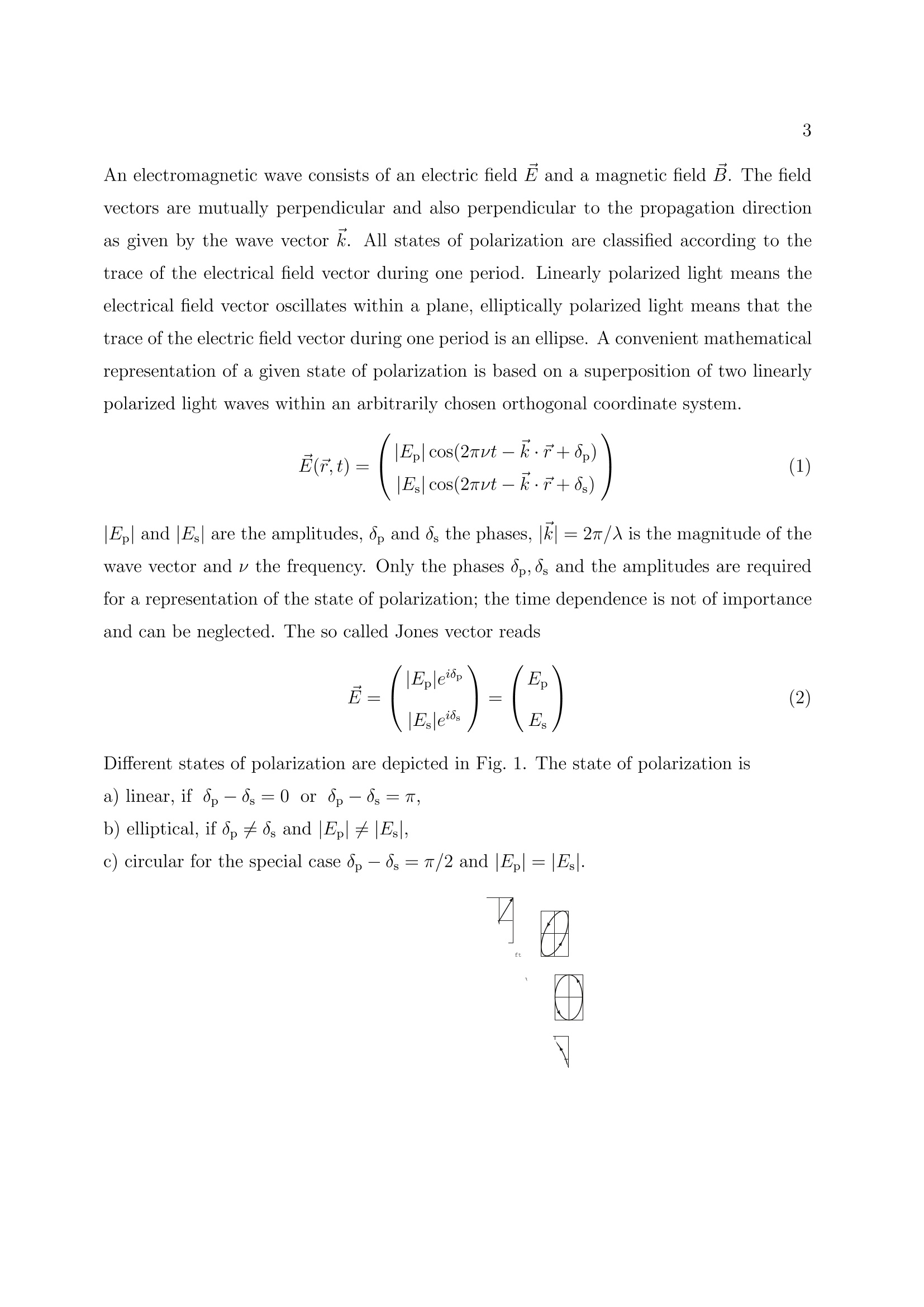
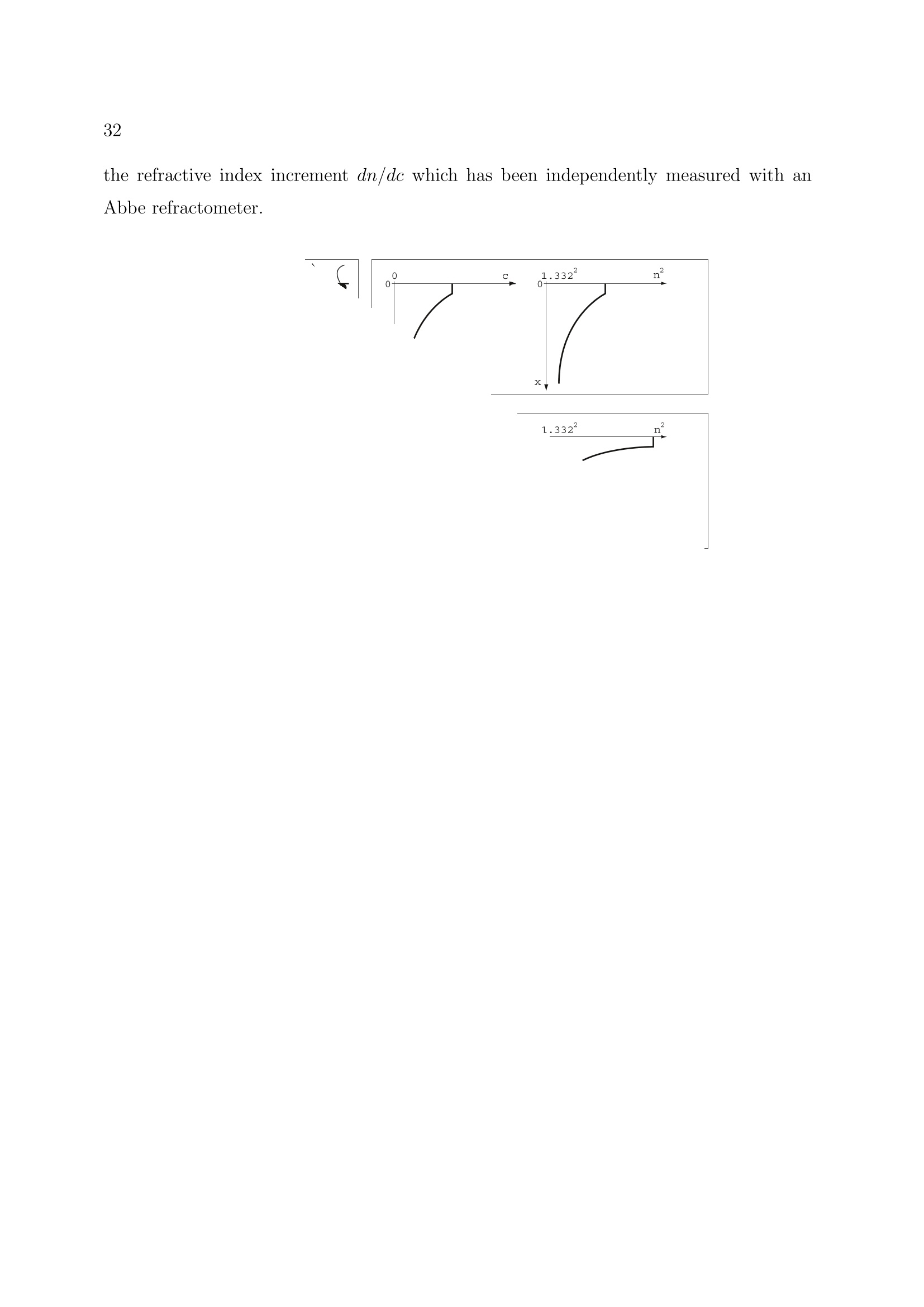
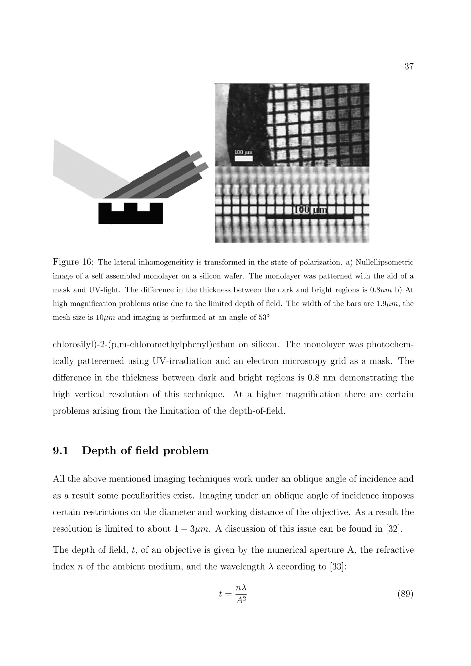
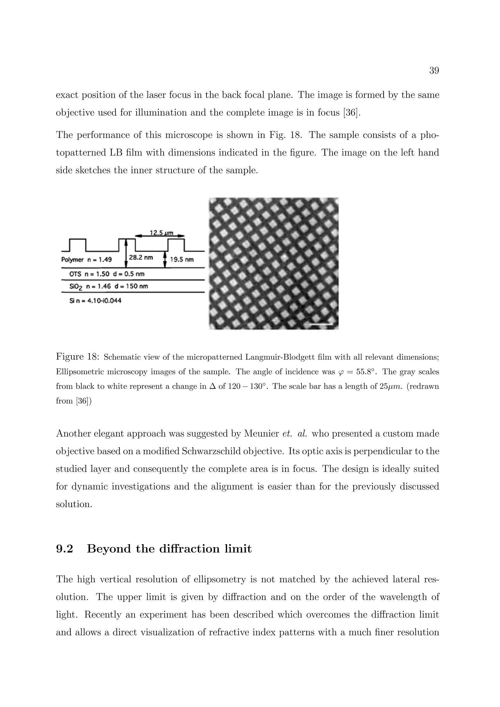
2 3 Ellipsometry in Interface Science H. Motschmann and R. Teppner Max-Planck-Institut fur Grenzflachenforschung, Golm Contents 1 What is it all about? 2 2 Polarized light 2 3 Basic equation of ellipsometry 5 4 Design of an ellipsometer 6 5Theory of reflection 10 6Ellipsometry applied to ultrathin films 17 7Microscopic model for reflection 19 8 Adsorption layers of soluble surfactants 23 8.1 Importance of purification 23 8.2 Physicochemical properties of our model systems 23 8.3 Adsorption layer of a nonionic surfactant. 24 8.4 Ionic surfactant at the air-water interface.. 25 8.5 Kinetics of absorption 34 9 Principle of imaging ellipsometry 36 9.1 Depth of field problem 37 9.2 Beyond the diffraction limit 39 1 What is it all about? The following chapter presents the basics of ellipsometry and discusses some recent ad-vances. The article covers the formalism and theory used for data analysis as well asinstrumentation..The treatment is also designed to familiarize newcomers to this field.The experimental focus is on adsorption layers at the air-water and oil-water interface.Selected examples are discussed to illustrate the potential as well as the limits of thistechnique. The authors hope, that this article contributes to a wider use of this techniquein the colloidal physics and chemistry community. Many problems in our field of sciencecan be tackled with this technique. Ellipsometry refers to a class of optical experiments which measure changes in the stateof polarization upon reflection or transmission on the sample of interest. It is a powerfultechnique for the characterization of thin films and surfaces. In favorable cases thicknessesof thin films can be measured to within A accuracy, furthermore it is possible to quantifysubmonolayer surface coverages with a resolution down to 1/100 of a monolayer or tomeasure the orientation adopted by the molecules on mesoscopic length scales. The highsensitivity is remarkable if one considers that the wavelength of the probing light is onthe order of 500 nm. The data accumulation is fast and allows to monitor the kinetics ofadsorption processes. The technique can also be extended to a microscopy. Imaging ellip-sometry allows under certain conditions a direct visualization of surface inhomogeneitiesas well as quantification of the images. Many samples are suitable for ellipsometry andthe only requirement is that they must reflect laser light. Its simplicity and power makesellipsometry an ideal surface analytical tool for many objects in interface science. 2 Polarized light Light is an electromagnetic wave and all its features relevant for ellipsometry can bedescribed within the framework of Maxwell’s theory [1]. The relevant material propertiesare described by the complex dielectric function e or alternatively by the correspondingrefractive index n. An electromagnetic wave consists of an electric field E and a magnetic field B. The fieldvectors are mutually perpendicular and also perpendicular to the propagation directionas given by the wave vector k. All states of polarization are classified according to thetrace of the electrical field vector during one period. Linearly polarized light means theelectrical field vector oscillates within a plane, elliptically polarized light means that thetrace of the electric field vector during one period is an ellipse. A convenient mathematicalrepresentation of a given state of polarization is based on a superposition of two linearlypolarized light waves within an arbitrarily chosen orthogonal coordinate system. |E,| and|E| are the amplitudes, , and o, the phases, |k|=2m/二 is the magnitude of thewave vector and v the frequency. Only the phases op,os and the amplitudes are requiredfor a representation of the state of polarization; the time dependence is not of importanceand can be neglected. The so called Jones vector reads Different states of polarization are depicted in Fig. 1. The state of polarization is b) elliptical, if 8,/og andE,/|Es|, c) circular for the special case op-二s=T/2 and|Epl=|Es|. An alternative representation of a given state of polarization uses the quantities ellipticityw and azimuth a. The ellipticity is defined as the ratio of the length of the semi-minoraxis to that of the semi-major axis as shown in Fig. 2. The azimuth angle a is measuredcounterclockwise from the s-axis. Light is assumed to propagate in positive 2 directionso thato, y and 2 define a right handed coordinate system. SSome authors prefer thisrepresentation and for this reason the conversion formulas between both notations arelisted below.The derivations require a vast number of tedious algebraic manipulationsand can be found in [2]. Ambiguities arising from the inversion of trigonometric functions are settled if the upperand lower limits of all quantities are considered. 3 Basic equation of ellipsometry A typical ellipsometric experiment is depicted in Fig. 3. Light with a well defined stateof polarization is incident on a sample. The reflected light usually differs in its state ofpolarization and these changes are measured and quantified in an ellipsometric experiment. Changes in the ratio of the amplitudes are described as the tangent of the angle亚. It willturn out later thatcan be directly measured. The reflectivity properties of a sample within a given experiment are given by the corre-sponding reflection coefficients r, and r. The reflection coefficient is a complex quantitythat accounts for changes in phase and amplitude of the reflected electric field E withrespect to the incident one E. Interference cannot be observed between orthogonal beams and hence p-and s-light donot influence each other and can be separately treated. With these definitions the basicequation of ellipsometry is obtained Eqn. (11) relates the quantities 亚 and A with the reflectivity properties of the sample.The following two section discuss various ways to measure ▲ and 亚 and the theory andalgorithm used for a calculation of the complex reflectivity coefficient. Some ellipsometersare designed in a way that they measure directly the real and imaginary part ofthe complexquantity p instead of and A. Eqn.(11) allows a conversion between both notations. 4 Design of an ellipsometer Many different designs of ellipsometers have been suggested and a good overview is pre-sented in Azzam and Bashara [3]. Here we discuss common roots of all arrangements andthe underlying theory. The layout of a typical ellipsometer is depicted in Fig. 4.The main components are apolarizer P which produces linearly polarized light, a compensator C which introduces adefined phase retardation of one field component with respect to the orthogonal one, thesample S, the analyzer A and a detector. Detector component coordinate system Jones-Matrix tp =transmission axisPolarizerep= extinction axis TC _10) The simple diagonal matrix is only valid in the coordinate system of the component. Amatrix R is required to transform the vector between the coordinate systems of adjacentcomponents. The setting of the optical components is defined by the angles P, A and C of its distinctaxis, with respect to the plane of incidence. An angle C=-45° means the fast axis ofthe compensator is set to an angle of -45°with respect to the plane of incidence. With these tools we can describe the E-vector at the detector as a function of the setting of all components including the unknown reflectivity properties of the sample. To understand Equation (14), one must first realize that the multiplication always goesfrom right to left. Hence, the above mathematical formula can be described as follows:linear polarized light exits the polarizer in the polarizer’s frame of reference, then is rotatedto the coordinate system of the compensator by the matrix operator R(C - P), then thecompensator acts on the state of polarization as given by Tc, then the exiting light fromthe compensator is rotated to the coordinate system of the sample by the matrix operatorR(-C) an so on. The multiplication given by Equation (14) yields: y accounts for the attenuation of the light intensity. Additional components in the opticalpath, for example the cell windows, should not change the state of polarization and cantherefore be neglected. The intensity at the detector is proportional to The Jones matrix algorithm leads to the desired relation between the intensity at thedetector and the setting of all optical components. The unknown reflectivity coefficientscan be retrieved in various manners and the applied measurement scheme names themethod.1.1Rotating analyzer means recording the intensity as a function of the settingof the analyzer and work out the unknown ellipsometric angles by a Fourier analysis.Polarization modulation ellipsometry uses a variable phase retardation , for a calculationof the ellipsometric angles. Polarization modulation uses an electro-optic or acusto-opticmodulator driven at a high frequency. The measurement is fast, however,there are alsosome inherent problems due to an undesired interferometric contribution of the modulatorto the signal which cannot be separated from the contribution of the sample. The techniqueis very well suited to follow relative changes. A particular successful implementation is Nullellipsometry which eliminates many intrinsicerrors due to slight misalignments of the sample. Within Nullellipsometry the setting ofthe optical components is chosen such that the light at the detector vanishes. This requiresthat the angle dependent term {Q1+22} of eqn. (15) vanishes. A given elliptical state ofpolarization of the incident light leads to linear polarized light after reflection and can becompletely extinguished with an analyzer. This equation can be further simplified by using a high precision quarter waveplate as acompensator (tc =1,8c=n/2= pc = -i) fixed to C=±45°. With eqn. (11) a furthersimplification of the eqn. (17) can be achieved. Eqn. (18) links the quantities ▲ an 亚to the null settings of the polarizePo and analyzerAo. Once a setting (Po, Ao) has been determined which provides a complete cancellationof the light, then the same holds for the pair(Po, Ao). These nontrivial pairs of nullsettings are refered as ellipsometric zones..Measurementsin various zones lead to a high accuracy in the determination of absolute values.Manvintrinsic small errors due to misalignment are cancelled by this scheme. So far we introduced two quantitites which account for changes in the state of reflectionupon reflection.We also discussed how these quantities can be measured.1.The nextchapter deals with the theory of reflection and illustrates means for a calculation of theellipsometric angles of a given optical layer system. 5 Theory of reflection In the following section a procedure for a calculation of the reflectivity coefficientsr, and rs(and consequently the ellipsometric angles) first published by Lekner [6] will be described. This method is certainly not the easiest one for the calculation of the reflectivity propertiesof a single homogenous layer at the interface between two bulk phases, but is advantageous,if the layer has an inner structure, e.g. a continuously varying refractive index normal tothe interfaces. For just a few refractive index profiles it is possible to calculate r, and rsexactly, but in most cases approximations must be used: A continuously varying refractiveindex profile is subdivided into many thin layers. This method uses matrices to relate theelectrical field and its derivative in between adjacent layer and matrices to account forchanges of the phase in each layer. In every layer the refractive index is assumed to beconstant. Obviously this approximation gets the better the finer the subdivision is. For the derivation we use a rectangular coordinate system with the 2-axis normal tothe interfaces pointing from the incident medium to the substrate.This means that theinterfaces of the layer structure are planes of constant 2n. The , 2-plane is the plane ofincidence. 0t with B representing the magnetic field, E the electric field, e(z)=n(z)" the dielectricfunction and c the velocity of light in vacuo. For the B- and the E-field a plane wave ansatz is used: This ansatz fulfills Maxwell's equations, if the following relationship between the wavevector k and the angular frequency w of the propagating wave is obeyed: and if additionally Bo, Eo and k are normal to each other. Thus eqn. (20) and eqn. (21)can be further simplified: Let’s consider s-polarized light, that can be represented in the following way in the coor-dinate system: Inserting Es in eqn. (26) results in three equations for E : After elimination of B and Bz one obtains a differential equation in E which can beseparated: The ansatz Ey(z,z,t)=e(kuz-wt). E(z) leads to a differential equation in E(z): with q being the 2-component of the wave vector: and y representing the angle of incidence (defined as the angle between the surface normaland the direction of propagation of the light beam). Since E(z) is continuous at everyinterface, it is obvious from eqn. (30), that also dE(z)/dz is continuous, if de /oo. Eqn. (30) can thus be split into two coupled differential equations of first order: If q takes the value qn within a layer located between 2n and zn+1, and En and Dn are thevalues of the electric field and its derivative at 2n, the solution of eqn. (32) in zn z≤2n+1is: Since E and D are continuous at the interfaces, it follows that with representing the phase shift encountered while propagating through the layer. The eqn. (35)can be expressed in a matrix form: where Mns describes the influence of the n-th layer on the s-polarized wave. The matrices for p-polarized light can be calculated analogously. Since p-light has non-vanishing s- and 2-components of the electrical field in the chosen coordinate system, it is more convenient to use the linearly coupled magnetic field B, which has just onenonvanishing component, instead of E. (38) Insertion of B into Maxwell’s equations and simplification lead to a differential equationin B(z): that can be split into two equations of first order again: Their solutions within a layer n resemble those of the s-polarized light (eqn. (33) andeqn. (34)): It follows from eqn. (20) and eqn. (39) that B(z) and C(z) are continuous at the layers'interfaces, if de o. This can be used again to relate the values of B and C at neighboringinterfaces. Now it is clear how to calculate the reflectivity coefficients of such a layer structure: Thelayers'matrices M, have to be multiplied consecutively, separately for p- and s-light: The resulting matrices M, and M, relate the fields before and after the layer structure. Before it (f)there are incident and reflected wave, behind it (h) just the transmitted one: (45) Thus the following relations evolve: These equations can be solved for r and rp, resulting in two formally identical expressionsfor the two coefficients: Up to now the only simplification is the discretization of the continuous refractive in-dex profile. The next step is a reduction of the computational effort by using a Taylor-approximation up to the second order in the phaseshift on. This approximation is valid ifthe discrete layer thicknesses are much smaller than the wavelength of the light: in otherwords a sufficiently high number of layers is required. for S- and p-polarized light simplify to With just a slight increase of computational effort the approximation can be greatly im-proved by using layers with linearly varying dielectric functions e as depicted in fig.6instead of those with constant e. 6 Ellipsometry applied to ultrathin films The previous section described an algorithm for the calculation on the reflectivity coeffi-cients of given refractive index profiles. Profiles are only of importance if their characteris-tic length scale is comparable to that of the probing beam. In many cases, i.e. adsorptionlayer of nonionic surfactants at the air-water interface, there is a striking mismatch be-tween interfacial height h and the wavelength of light 入. As a result certain peculiaritiesexist which are discussed in this section [8]. The most striking limitation is a reduction of the measurable quantities. The presenceof an organic monolayer (refractive index 1.3-1.6) with a thickness below 2.5 nm doesnot change the reflectivity |ri2and as a consequence there are no detectable changes in.. In the thin film limith <入the data analysis relies only on a single parameter,namely changes in the phase . Unfortunately the number of independent data cannotbe increased. Neither spectroscopic ellipsometry nor a variation of the angle of incidenceyield new independent data, instead all quantities remain strongly coupled. A soundtreatment is given in [9]. However, the sensitivity of an ellipsometric measurement canbe significantly increased by the choice of the angle of incidence. A sensitivity analysis isgiven in 10. The exact formula relating the reflectivity coefficients of a single homogeneous layer withrefractive index n1 =√e in between two infinite media (no=√o and n2=√6) at anangle of incidence y is given by : where the reflectivity coefficients ro,1,p; T1,2,p; ro,1,s and r1,2,s describing the reflection atrefractive index jumps no→n一 and n1→n2 for p- and s-light are given by Fresnel’s laws.3=2m²√n?-n?sin?yaccounts for the phase shift occuring in a single pass within theadsorption layer. If the layer thickness h is much smaller than the wavelength 入 of light it is justified toexpand the complex reflectivity coefficients in a power series in terms of h/. The first term in this expansion describes reflection at a monolayer. If the refractive index is varying over the height of the layer, the term within eqn. (63) has to be replaced by an integral n across the interface: An ellipsometric experiment on a monolayer yields a quantity proportional to n. A sim-plification of eqn. (55) reveals its physical meaning. Quite often, as for example in caseof adsorption of organic compounds onto solid supports 7], E2 exceeds e of the monolayerwhilee≈ 6o Under these circumstances eqn. (55) can be further simplified: A linear relationship between e and the prevailing concentration c of amphiphile withinthe adsorption layer is well established [11] This relation yields a direct proportionality between the quantity n and the adsorbedamount T. None of the assumptions which lead to eqn. (58) apply for adsorption layers at the liquid-air interface and hence eqn. (55) cannot be further simplified. The relationship betweenmonolayer data and recorded changes remains obscure with no further simplificationspossible on the basis of Maxwell’s equations. A proportionality between A and I mayhold but it cannot be established within this theoretical framework. 7 Microscopic model for reflection Quantities such as refractive index or thickness are macroscopic quantities. Their meaningat sub-monolayer coverage is not an obvious one.To bridge these inherent difficultiesseveral approaches have been developed aiming for a calculation of the optical propertiesof a monolayer based on microscopic quantitities [12]. We follow here mainly a modeloriginally derived by Dignam et.al.. [13, 14]. Explicit formulas are derived relating thechanges in ▲ to the polarizibility tensor of the adsorbed molecule and their number densityat the interface. The adsorption layer is treated as a two dimensional sheet of dipoles driven by the externallaser field. The oscillating dipoles act as sources of radiation and the summation of alltheir contributions yields the reflected beam in the far field. The adsorption layer is considered as homogeneous, fluctuations in the orientation ordensity occur on a length scale much smaller than the wavelength of light. These conditionsare usually fulfilled for adsorption layers of soluble surfactants. The decisive new quantitity introduced by Dignam et.al. is the surface susceptibilitytensor which links the external electric field Eo to the resulting polarization per volume P, trepresents the thickness of the adsorbed layer. The polarization is given by the vectorsum of all dipole moments uj over all molecules j: The local field at each dipole has two origins, the external laser field Eo and the dipolarcontribution which is proportional to Eo. Each adsorbed molecule is characterized by its own tensor B. The induced dipole momentof a molecule with a polarizability a; is given by with this notation the susceptibilty tensor y reads: In order to calculate f it is desirable to introduce the field Eij, which accounts for theelectric field at the position ri generated by the dipole of molecule j. The projection operator p projects the induced dipole moment on the connection of themolecules at site i and j. With the relation: B, is given by Each molecule is characterized by a tensor B. For a further calculation certain assumptionsabout the molecular distribution must be introduced. For adsorption layers of solublesurfactants at the air-water interface it is a good approximation to consider B for allmolecules equal. The underlying molecular pircture is is that the adsorption layer consistsof one species of amphiphiles with a narrow angular distribution. Under these conditions: meaning that With equation 63 the surface susceptibility tensor reads: The number of molecules per unit area is denoted by N. For an uniaxial film with itsoptical axis parallel to the surface normal the tangential t and normal n component of thesusceptibility tensor read: The quantity te can be regarded as an effective thickness as defined as If the adsorption layer can be mathematically represented as adsorbed molecules on arectangular grid with an average next neighbour distance of a At monolayer coverage N = 1/athe effective thickness is te=0.935a. The adsorptionof molecules at the interface changes the optical properties of the system. The changes inthe ellipsometric angles are given by In the thin film limit only changes in A occur: oYn,t denotes the difference of the susceptibility tensor between the film covered and thebare surface,i =√-1, p is the angle of incidence and 入 is the wavelength of light.Changes in the ellipsometric angle ▲ are given by the difference in L parallel and perpen-dicular to the plane of incidence. The parallel component reads whereas the perpendicular component is given by This model reflects the optical response at the molecular level, but the model suffers fromits complexity and high number of parameters, the values of which can only be assumed.Since the macroscopic ansatz resulting in eqn. (54) comes to similar results with a properlychosen dependence of the refractive index of the layer on the adsorbed amount, the use ofthe microscopic model is not common in practical applications. In the following sectionwe will discuss some representative examples. 8 Adsorption layers of soluble surfactants 8.1 Importance of purification Due to the peculiarities of surfactant synthesis, many surfactants contain trace impuri-ties of higher surface activity than the main component..T.hese trace impurities do notinfluence most bulk properties. However, at the surface they are enriched and impuritiesmay even dominate the properties of the interface.. This behaviour was first recognizedby Mysels [15] and a purification scheme using foam fractionation was proposed [16]. Adetailed discussion on artifacts caused by impurities can be found in [17]. In studies performed in our lab, we use a fully automated purification device developed byLunkenheimer et. al. which ensures a complete removal of these unwanted trace impurities[18]. The aqueous stock solution undergoes numerous of purification cycles consisting ofa) compression of the surface layer, b) its removal with the aid of a capillary, c) dilation toan increased surface and d) formation of a new adsorption layer. At the end of each cyclethe surface tension ae is measured. The solution is referred to as surface chemically puregrade if oe remains constant in between subsequent cycles. Quite frequently more than300 cycles and a total time of several days are required to achieve the desired state. Thesample preparation is time consuming and tedious but mandatory for the investigation ofequilibrium properties of adsorption layers of soluble surfactants at the air-liquid interface. 8.2 Physicochemical properties of our model systems In the following we discuss the interfacial properties of two related amphiphiles, thecationic amphiphile 1-dodecyl-4-dimethylaminopyridinium bromide, C12-DMP, and theclosely related nonionic 2-(4'dimethylaminopyridinio)-dodecanoate, C12-DMP betaine.The corresponding chemical structures are depicted in fig.7 together with their equi-librium surface tension isotherms. The synthesis is described in 19]. Both components are classical amphiphiles and resemble all common features such as theexistence of a critical micelle concentration cmc. The members of the homologous seriesof the alkyl-dimethylaminopyridinium bromide are strong electrolytes and follow the pre- dictions of Debye-Hickel theory as experimentally verified by conductivity measurements.For solubility reasons we used 1-butyl-4-dimethylaminopyridinium bromide instead of theC12 representative of the homologous series which gave us experimental access to a widerconcentration range. Debye-Hiickel predicts a proportionality of the activity coefficientto the square root of the ionic strength for aqueous solutions of 1:1 electrolytes which isindeed observed in our experiment. I is then compared to the changes of the ellipsometric quantity ▲-Ao. The inset of Fig. 8presents the result. The surface excess as given by the slope of the surface tension isothermis compared to the ellipsometric response at each concentration. Obviously the relationbetween both quantities can be described by a straight line. Hence, experimental evidencehas been provided that ellipsometry measures indeed the surface excess of the adsorptionlayer of the soluble nonionic amphiphile. Since optics measures refractive indices whichare not very sensitive to molecular details we anticipate that this holds for a wider classof materials. ment carried out on adsorption layers of an ionic surfactant. It will be demonstrated thatthere are major differences between the two model systems. The adsorption layer is described as an isotropic optical layer of constant thickness with arefractive index nlayer which depends on the surface coverage [21]. Within this model thereare two distinct surface concentrations which lead to a vanishing dA=A-A0=0°. Atvery low coverage the refractive index of the layer matches the one of air nayer = nair =1and at an intermediate surface coverage the surface layer adopts the very same refractiveindex as the water bulk phase nayer= n=wateerr = 1.332. Consequently there has to bean extremum in between.The resulting dA(nlayer)-curve is depicted in Fig. 10.Thegeometrical dimension of the molecules has been used as thickness of the layer. Scenario 2: Effect of anisotropy The following provides an estimation if changes in the molecular orientation may be respon-sible for the surprising features in the ellipsometric isotherm. The following assumptionswere made in order to estimate an upper limit for this effect: ●The optical model is that of an uniaxial layer with the optical axis normal to theinterface. The molecular arrangement is Coov which has been experimentally verifiedfor the headgroups by polarization dependent SHG measurements. ●The thickness of the adsorbed layer and the mean tilt angle of the molecules withinthe layer change with their number density N at the interface. Within the investi-gated number density range the thickness increases from 1nm to 1.9nm proportionalto the cosine of the tilt angle which is assumed to change from around 70° to 40°. ●The whole molecule, including the head group, is assumed to change its tilt angle.The molecules are assumed to be all-trans and perfectly aligned which would yieldthe maximum possible change in anisotropy. ●The refractive index for an E-vector along the length axis of the molecule is naris =1.56, while the refractive index for an E-vector perpendicular to the long axis ofthe molecule is nperp =1.48. Both refractive indices have been taken from Riegleret.al. 22 and rely on a combination of X-ray reflection data with ellipsometricmeasurements of monolayers of behenic acid at the air-water interface for a denselypacked and perfectly oriented apmphiphiles. In our case the actual refractive indiceswill depend on the prevailing volume concentration and the data are therefore anupper limit. The calculated dA(N) versus density-curve is plotted in Fig. 11. Obviously a change ofthe molecular tilt leads to changes in dA, but cannot account for the measured pronouncedextremum. In addition it is impossible to reach dA=-2.77°, which is the minimum ofthe measured curve, with reasonable parameters for the anisotropic layer. An increasein anisotropy has the same impact on the ellipsometric measurements as a reduction of Scenario 3: Changing the counterion distribution Ellipsometry probes the complete interfacial architecture. The reflected light is generatedwithin the transition region between the two adjacent bulk phases, air and aqueous surfac-tant solution. The electric double layer has to be explicetely considered. Hence, changesin the ion distribution at higher concentrations may cause the observed feature in theellipsometric isotherm. The classical model of a charged double layer has been developed by Gouy, Chapman andStern. The interface is described by two distinct regions: a compact layer consisting ofthe positively charged adsorbed amphiphiles with some directly adsorbed counterions anda diffuse layer of counterions. The ion distribution within the diffuse layer is given by the solution of the Poisson equationwhich relates the divergence of the gradient of the electric potential 重 to the charge densityp at that point (see for instance [23, 24]): The compact layer is positively charged and in contact with an electrolyte solution whichforms a diffuse layer of charges. The ion concentration distribution within the electricalpotential obeys Boltzmann: where z and z+ are the valencies of the anions and cations respectively. For a symmetricelectrolyte solution (-z- = z+=二 and c, =c, = co) eqn.(84) leads to a net charge ofthe ion cloud of The combination of eqn.(85) with the Poisson eqn.(83) yields a differential equation in theelectric potential. In our case the potential is only a function of the normal coordinateto the surface s. It is convenient to define a reduced potential which further simplifies the equations and results in The integration of equation (87) with the boundary conditions (y=0 and dy/ds =0) for= oo and y=y, at x = 0 lead to the Gouy-Chapmann solution of the reduced potentialwithin the diffuse layer: Hence, knowing the charge of the compact layer the ion distribution can be modelled. Thecrux of Stern’s treatment is the estimation to which extent ions enter the compact layerand reduce the surface potential. The ion distribution between compact and diffuse layercannot be easily experimentally established, for example surface potential measurementscannot measure this distribution. The optical analysis requires the translation of the prevailing distribution of moleculesand ions within the interphase into a corresponding refractive index profile. The reflec-tivity coefficients can then be calculated on the basis the previously discussed numericalalgorithms for stratified media. Two elements dominate the refractive index profile andhence the reflectivity properties, the topmost monolayer of the amphiphile and the distri-bution of ions within the diffuse layer. The excess of ions within the diffuse layer leadsto a slightly elevated refractive index as compared to the bulk of the aqueous surfactantsolution. The typical dimensions of the diffuse layer are on the order of 10 nm and thisfairly wide extension leads to a profound impact on A, since the topmost monolayer hasa normal extension of only 2 nm. The solution of the potential重plugged into equation(85) yields the distribution of anions and cations within the diffuse layer. The prevailingcharge distribution is determined by the surface charge of the topmost monolayer. Therefractive index profile is then determined by the ion distribution by a multiplication with the refractive index increment dn/dc which has been independently measured with anAbbe refractometer. excess. It is therefore a valuable alternative to surface tension measurements, especially ifone considers rheological properties which require higher derivatives of the surface tensionisotherm. 8.5 Kinetics of absorption Rapidly expanding liquid surfaces occur in many technical processes such as foam forma-tion, spraying or painting, they are also omnipresent in nature, i.e. the oxygen exchangein the lung. Surfactants play a crucial role in these processes.They stabilize the newsurfaces by a reduction of the surface tension. Inhomogeneities in surface coverage leadto gradients in surface tension which in turn have a strong impact on bulk hydrodynamicflow, a phenomenon also known as Marangoni flow. The overall dynamic behaviour isvery complex and despite many efforts far from understood [25]. The investigation re-quires time resolution within the ms regime putting severe limitations on the choice ofthe experimental technique..ThTe maximum bubble pressure method [25] is most oftenused to perform these types of studies but ellipsometry offers an interesting alternativeto supplement these investigations. This method relies on surface tension measurementsand the surface coverage is obtained using the equilibrium surface isotherm. The under-lying assumption is that the surface is locally at equilibrium, however, in the time regimeof interest this may not be the case. As outlined in the theoretical section ellipsometrymeasures directly the surface coverage for nonionic surfactants and provides in additionthe requested time resolution. The challenging part is the design of an experiment withprecisely defined boundary conditions required for modeling the underlying physics lead-ing to the observed kinetic behavior. The most promising approaches produce an interfacewith a non-equilibrium surface coverage, and maintain that surface coverage through theflow of fluid in and out of the control volume. To satisfy the requirement of well-definedboundary conditions, at the beginning of the flow a freshly formed surface must be created.Several arrangements have been suggested such as the inclined plate [25], the overflowingcylinder [26] or the use of a jet [27]. In all these approaches the surface has a defined ageat a given spot, hence the desired dynamic picture of the surfactant adsorption is obtainedby moving the sample relative to the light beam. ▲ ◆A ▲ Figure 16: The lateral inhomogeneitity is transformed in the state of polarization. a) Nullellipsometricimage of a self assembled monolayer on a silicon wafer. The monolayer was patterned with the aid of amask and UV-light. The difference in the thickness between the dark and bright regions is 0.8nm b) Athigh magnification problems arise due to the limited depth of field. The width of the bars are 1.9pm, themesh size is 10pm and imaging is performed at an angle of 53° chlorosilyl)-2-(p,m-chloromethylphenyl)ethan on silicon. The monolayer was photochem-ically pattererned using UV-irradiation and an electron microscopy grid as a mask. Thedifference in the thickness between dark and bright regions is 0.8 nm demonstrating thehigh vertical resolution of this technique. At a higher magnification there are certainproblems arising from the limitation of the depth-of-field. 9.1 IDepth of field problem All the above mentioned imaging techniques work under an oblique angle of incidence andas a result some peculiarities exist. Imaging under an oblique angle of incidence imposescertain restrictions on the diameter and working distance of the objective. As a result theresolution is limited to about 1-3pm. A discussion of this issue can be found in 32. The depth of field, t, of an objective is given by the numerical aperture A, the refractiveindex n of the ambient medium, and the wavelength 入according to 33: Depending on the angle of incidence, p,and the numerical aperture, A, only a region ofthe illuminated part of the sample is in focus.This region is of the order of 1 - 50um.This problem is illustrated in Figure (16b). The size of a bar is 1.9um, the mesh size is10pm and imaging was performed at p=53°. The depth-of-field problem is a severe limitation at higher magnification. A straightfor-ward solution consists of a scan of the objective 34]. Only the area in focus is recordedand the complete image is constructed by many stripes by imaging processing software.This procedure yields sharp images of static objects. At the oil-water or air-water interfaceit is only of limited use due to the prevailing convection. Figure 17: Principle of ellipsometric microscopy. Full arrows symbolise the light path of illumination,broken arrows stand for the observation, respectively. A parallel beam of polarised light is focussed intoan off-axis spot in the back focal plane of the lens. In the front focal plane of the lens, where the objectis located, this results in a parallel polarised beam of light hitting the object under a shallow angle ofincidence. Light reflected by the object is collected by the lens, passes a motorised polarization analyzerand is focused onto a digital CCD camera. For clarity, several optical elements are omitted. (redrawnfrom 36) An elegant approach which overcomes these difficulties was suggested in the group ofSackmann et al.. A parallel polarized laser beam was focused to an off axis spot in theback focal plane of a microscope objective of high numerical aperture. The sample which islocated in the front plane is then illuminated by a parallel polarized beam of light incidenton the sample under an oblique angle. The exact angle of incidence is controlled by the exact position of the laser focus in the back focal plane. The image is formed by the sameobjective used for illumination and the complete image is in focus [36]. The performance of this microscope is shown in Fig. 18. The sample consists of a pho-topatterned LB film with dimensions indicated in the figure. The image on the left handside sketches the inner structure of the sample. Figure 18: Schematic view of the micropatterned Langmuir-Blodgett film with all relevant dimensions;Ellipsometric microscopy images of the sample. The angle of incidence was p= 55.8°. The gray scalesfrom black to white represent a change in ▲ of 120-130°. The scale bar has a length of 25um. (redrawnfrom 36]) Another elegant approach was suggested by Meunier et. al.who presented a custom madeobjective based on a modified Schwarzschild objective. Its optic axis is perpendicular to thestudied layer and consequently the complete area is in focus. The design is ideally suitedfor dynamic investigations and the alignment is easier than for the previously discussedsolution. 9.2 Beyond the diffraction limit The high vertical resolution of ellipsometry is not matched by the achieved lateral res-olution. The upper limit is given by diffraction and on the order of the wavelength oflight. Recently an experiment has been described which overcomes the diffraction limitand allows a direct visualization of refractive index patterns with a much finer resolution [37]. The arrangement is based on a combination of Atomic Force Microscopy (AFM) andEllipsometry and the AFM tip dimensions determines the resolution. The sample of interest is mounted on the base of a prism. The ellipsometer is operatedin the null mode and the total reflected light at the prism base is completely cancelled bythe setting of the polarization optics. This null setting is kept constant during the courseof the experiment. The metal AFM tip couples to the evanescent field and depending onthe local optical properties of the sample the null setting is out of tune. The intensityat the detector is monitored while carrying out a topographic scan with a conventionalAtomic Force Microscope. Thus two images are simultaneously generated: a topographicimage by the AFM tip and an ellipsometric image which relates the intensity reading atthe detector with the x,y position of the tip. The latter contains information on refractiveindex inhomogenity. This technique allowed for instance a visualization of 10 nm CDTeparticles within a polymer matrix.The topographic scan was not able to identify theparticles within the spincoated polymer film. However, due to the differences in therefractive index it could be visualized by the ellipsometric image. isator zer im References [1] M. Born, Optik, Springer Verlag, New York, Heidelberg (1998) [2] D. S. Kliger, J. W. Lewis, C. Randall, Polarized Light in optics and spectroscopy,Academic Press, Harcout Brace Javanovich Publishers, Boston (1990) [3] R. M. Azzam, N.M. Bashara, Ellipsometry and Polarized Light,North Holland Publication, Amsterdam (1979) [4 R.C. Jones, J. Opt. Soc. Am 16, 488 (1941) ( 5] S.N. Jasperson, S.E. Schnatterly, R eu. S ci. I nstr. 40, 761 (1 9 69) ) ( [6] J. Lekner, Theory of Reflection, Martinus Nijhoff Publishers, Boston, ( 1987) ) ( [7] T . K ull, T. Nylander, F. Tiberg, N. Wahlgren, Langmuir 1 3 , 5141 (1997) ) ( [8] R. Teppner, S . Bae, K. Haage, H . Motschmann, Langmuir 15, 7 002 ( 1999) ) ( [9] R. Reiter, H. Motschmann, H. Orendi, A. Nemetz, W. Knoll, Langmuir 8, 1784 (1992) ) ( [10] C. Flueraru, S. Schrader, V. Zauls, H. Motschmann, Thin Solid Fi l ms 379, 15 (2000) ) ( [11] H. Motschmann, M . Stamm, C . T o prakcioglu, M acromolecules 24, 3 681 ( 1991) ) ( [12] J. Lekner, P.J. Castle, Physica 101A, 89 ( 1 980) ) ( [13] M.J. Dignam, M. M o skovits, J. Chem. Soc. Faraday II 6 9, 56 (1973) ) ( [14] M.J. Dignam, J. Fedyk, J. Phys. (Paris) 3 8 , C5-57(19 7 7). ) ( [15] P.H. Elworthy, K .J. M ysels, J. Coll. I nt. Sci. , 331 (1966) ) ( [16] K.J.Mysels, A . Florence, J. Coll. Int. Sci. 43,57 7 (1973) ) ( [17] K. Lunkenheimer, J . Coll. Int. Sci. 131 , 580 (1989) ) ( [18] K. Lunkenheimer, H . J. Pergande, H. Kriger, Reu. Sc i . Instr. 58, 2313 ( 1 987) ) ( [19] K. Haage, H. Motschmann, S. Bae, E. Griindemann, Colloids a n d Surfaces ( i n press) ) ( [20] R. Teppner, K. Haage, D. Wantke , H. Motschmann,J.Phys.Chem.B 104, 11489 (2000) ) 21T. Pfohl, H. Mohwald, H. Riegler, Langmuir 14,5285(1998)22 M.Paudler, J. Ruths, H. Riegler, Langmuir 8, 184 (1992) [23] D.F. Evans, H. Wennerstrom, The Colloidal Domain,VCH Publishers, New York (1994) [24 A.W. Adamson, Physical Chemistry of Surfaces, Wiley & Sons, New York (1993) [25] S.S. Dukhin, G. Kretzschmar, R. Miller,Dynamics of Adsorption at Liquid Interfaces, Elsevier, Amsterdam (1995) [26] D.J.M. Bergink-Martens, H.J. Bos, A. Prins, B.C. Schulte, J. Coll. Int. Sci. 138(1990); D.J.M. Bergink-Martens, H.J. Bos, A. Prins, J. Coll. Int. Sci. 165, 221 (1994) ( 27 B . A. Noskov, Ad u . Co l loid In t erface Sci. 69, 63(1996) ) [28] S. Manning-Benson, S. R. W. Parker, C. D. Bain, J. Penfold, Langmuir 14,990(1998) ( [29] J. Hutchiso n , D. Klenerman, S. Manning-Benson, C. Bain, L angmuir 15, 7530 (1999) ) ( 30] A .F.H. Ward, L. Tordai, J. C h em. Phys. 14, 453 (1946) ) ( 31] D . Honig, D . M obius, J. P hys. Chem 95,4590 (1991) ) ( [32] M. Harke, R. T eppner, O. Schulz, H. Orendi, H. M o tschmann,Rev. Sci. Instrum. 68,8,3130 (1997) ) ( [33] H. Riesenberg H andbook of Microscopy, V E B Verlag Technik, Ber l in (19 88 ) ) ( 34 S . Henon, J . Meunier, Rev. Sci. Instr. 62,936 (1991) ) ( [35] M. Losche, E. Sackmann, H. M ohwald, Ber. Bunsenges. Ph y s. Ch e m. 10,848 (1983)[36] K.R. Neumaier, G. E lender, E. Sackmann, R. Merkel, ) ( Europhysics L etters 49 (1), 14 (2000) ) ( [37] P. Karageorgiev, H . Orendi, B. Stiller, L . B r ehmer, Appl. Phy s . Lett., (2001) in p r ess )
确定


还剩40页未读,是否继续阅读?


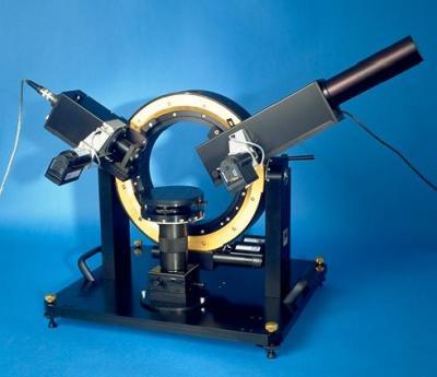
北京欧兰科技发展有限公司为您提供《界面和表面科学中椭偏分析方法检测方案(椭偏仪)》,该方案主要用于其他中椭偏分析方法检测,参考标准--,《界面和表面科学中椭偏分析方法检测方案(椭偏仪)》用到的仪器有组合式多功能椭偏仪
相关方案
更多
该厂商其他方案
更多