浅水流动表面中速度场检测方案(粒子图像测速)

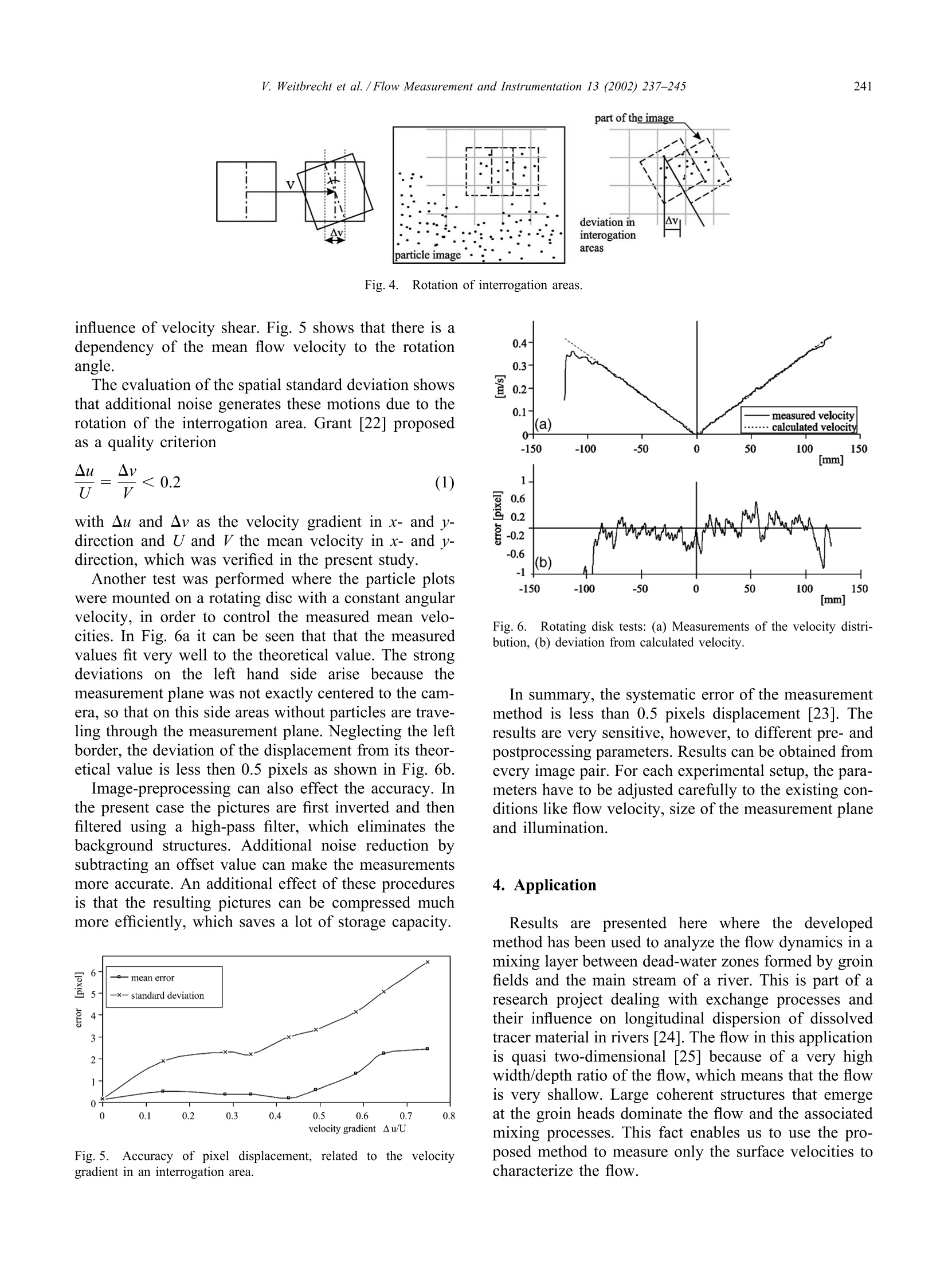
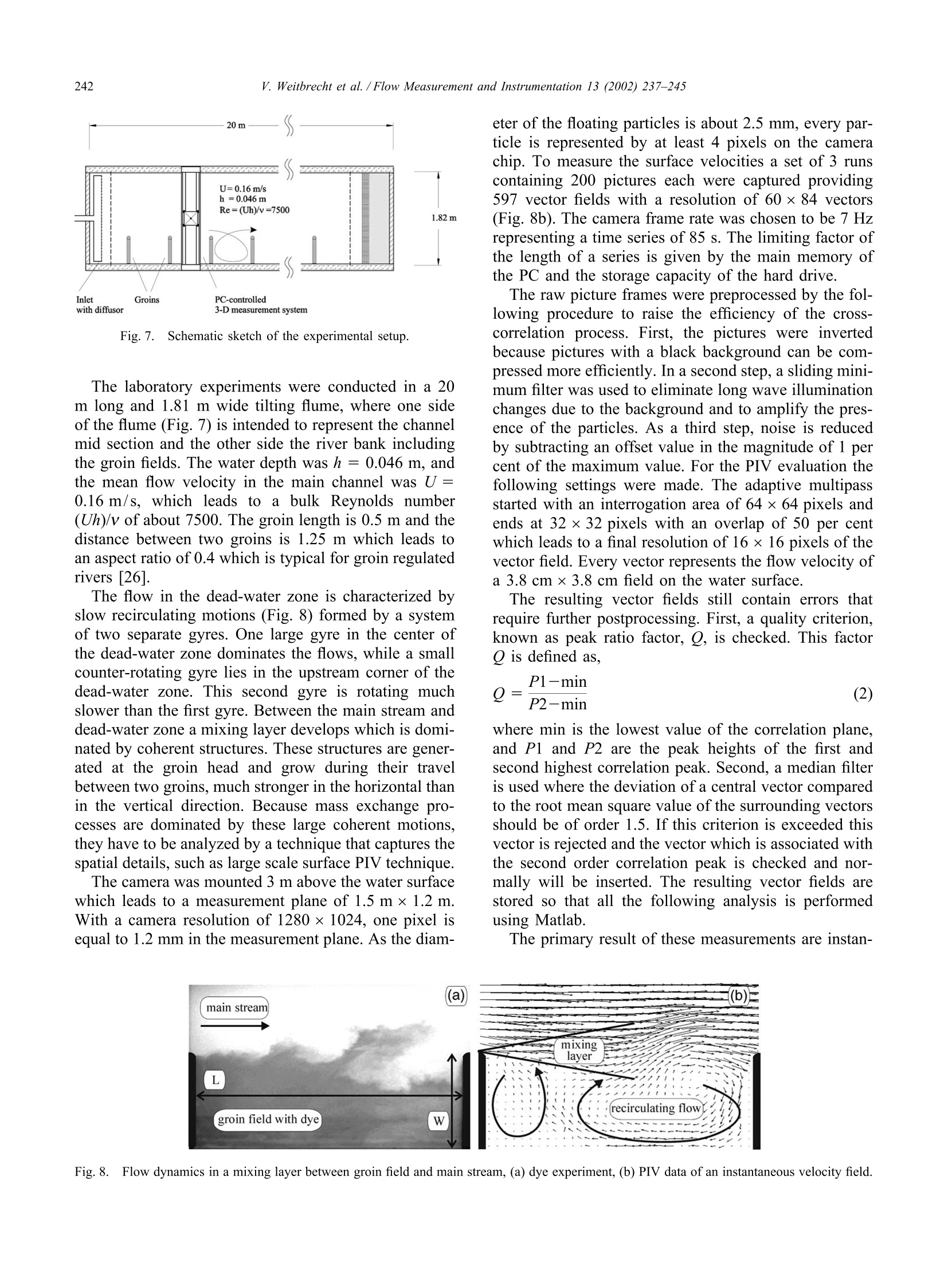
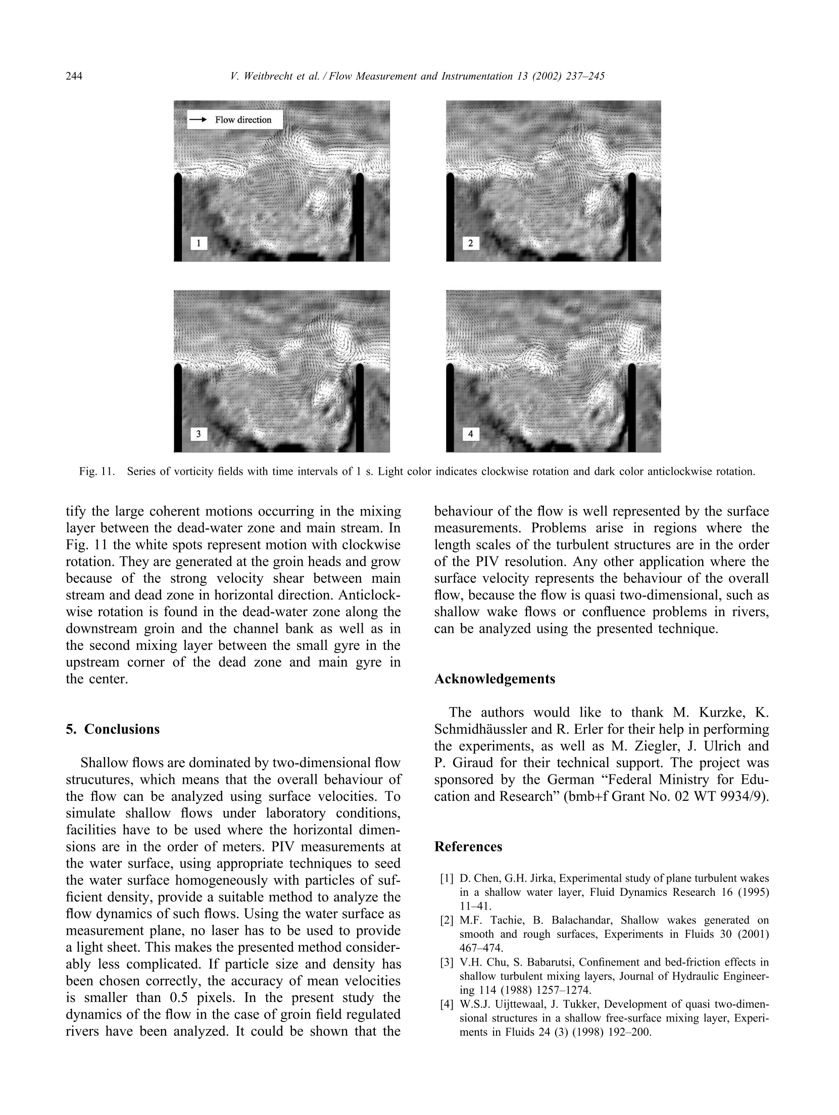
NowMeasurementand InstrumentationFlow Measurement and Instrumentation 13 (2002) 237-245www.elsevier.com/locate/flowmeasinst 238V. Weitbrecht et al. /Flow Measurement and Instrumentation 13 (2002) 237-245 Large scale PIV-measurements at the surface ofshallow water flows V. Weitbrecht *， G.Kihn，G.H. Jirka Institute for Hydromechanics， University ofKarlsruhe， 76128 Karlsruhe， Germany Abstract To measure the flow dynamics at the surface of shallow water flows over a large measuring field， a simple and reliable methodhas been developed using the advantages of Particle Image Velocimetry (PIV). Besides the determination of mean flow conditionsand turbulent flow characteristics， this method makes it possible to track two-dimensional large coherent structures， which are thedominating flow phenomena in many shallow flow applications. As basic equipment， a commercial PIV software system has beenused. The measurements are carried out at the water surface， which means that no laser light sheet is needed. Depending on thetime scales of the flow and camera characteristics， it is even possible to work with a constant light source. A particle dispenser topro de geneous distribution of particles on the water surface is also presented. Because floating particles have a strongtendency of sticking together， different types of particles and special coatings have been tested to reduce this problem. A laboratoryapplication of this method is presented to analyze the effects of shallow dead-water zones on exchange processes in rivers wherelarge coherent two-dimensional flow structures in the mixing layer dominate the flow characteristics. O 2002 Elsevier Science Ltd. All rights reserved. Keywords： Large scale PIV； Shallow flows； Grain fields； Particle dispenser 1.Introduction In shallow flow problems velocity information withhigh spatial and temporal resolution is needed to under-stand the dynamics of the flow and the related mixingprocesses. Shallow flow phenomena can be found in riv-ers， coastal zones or the atmosphere， where the dominat-ing processes are two-dimensional [1]. Large coherentmotions， that are inititated， for instance， in shallow wakeflows behind obstacles [2] or in shallow mixing layers[3-5] strongly influence the dynamics of such a systemand are， therefore， a determining factor for the mixingand transport processes. Measurement of the velocityfield describing the generation and the evolution of thesecoherent motions is the major aim of this investigation. To simulate shallow flows under laboratory con-ditions， scaling effects limit the minimum dimensionsand velocities such a model may have. For example， itit necessary that viscous forces do not influence the flow ( * Corresponding author. Tel.： +49(0)721/6087682； fax： +49(0)721/661686. ) ( E-mail address： weitbrecht@ifh.uka.de (V . We i tbrecht). ) much more than in the natural flow. This restriction leadsto scale models where the measurement area is on theorder of meters. The fundamental properties of shallow flows can beobtained by measuring surface velocities because of thetwo-dimensional behaviour of these flows. Moreover，the horizontal length scales of the coherent structures inthese flows are much larger then the vertical extent ofthe flow， which means that the dominating processes arein the horizontal plane. The flow structure in verticaldirection of shallow flows can be determined using themeasured surface velocities and adapting known verticalvelocity profiles， such as those determined by Blasiusfor open channel flow [6]， or for turbulent jets in shallowwater 71. In the present study PIV has been used to measurevelocity fields at the water surface. PIV constitutes apowerful technique to perform two-dimensional quanti-tative measurements for a large variety of flows [8，9].Many investigations have been made to improve the per-formance of PIV in the past by developing new corre-lation methods [10] or improving the image processing[11]. These efforts have lead to “off the shelf’PIV-pack-ages that are easy to adapt for different application. Compared to standarddPIVapplicationswheremeasurements are carried out within the water bodyusing a laser light sheet to illuminate the measuringplane [12-14]， surface PIV measurements are relativelystraightforward because no laser is needed. In this casethe measuring plane is given by the water surface whichmeans that for illumination， standard flood lights can beused， provided that the water surface is not strongly dis-turbed by wave motions. To keep the developed systemflexible， a commercial PIV package including camera，frame grabber， and controlling and evaluation softwarehas been used， with special adaptation to the large scalelaboratory problem. PIV measurements in large measur-ing areas have been performed in former investigationsby Linden et al. [15] and Tarbouriech et al. [16] in rotat-ing tanks with stratified flow conditions. In both casesthe measurements have been performed using a lightsheet to illuminate the measuring plane. Uijttewaal [17]presented particle tracking measurements at the watersurface where the particles were distributed manually onthe water surface. In Uijttewaal et al. [18]， measurementscan be found using the presented method， where theinfluence of grid turbulence on shallow flows weredetermined. Von Carmer et al. [19] were using thepresented technique to analyze shallow wake flows. Measurements of velocity fields in large areas withhigh spatial and temporal resolution are difficult becauseof the problem of homogeneous particle seeding on thewater surface. To solve this problem a particle dispenser(see Section 2) has been developed which can bemounted a short distance upstream of the measurementarea over the water surface. A second major problemrelates to the tendency of most floating particles toagglomerate. This phenomena leads to a distorted par-ticle distribution which means that in some regions noparticles are found while in other regions large particleaggregations are floating on the water surface. A study ofdifferent particle materials and special coatings to reduceagglomeration is presented in Section 2. In Section 3the results are given of different tests that evaluate theaccuracy of the presented method. In Section4 measurements are presented where thesystem has been applied to a laboratory problem. Inthese experiments exchange processes between dead-water zones and the main stream of a river have beeninvestigated to determine the influence of these zones onthe transport characteristics of the river. First， the meanflow conditions are presented to visualize the recirculat-ing water body. Second， the turbulent motion rep-resenting the fluctuating part of the water motion arepresented in order to characterize the mixing layerbetween the dead-water zone and the main stream.Finally， vorticity fields to analyze the coherent motionof the flow in the mixing layer are determined. 2. Elements of the measuring system In the following section the different parts of the mea-suring system， PIV-package， camera， particles， particledispenser， and illumination， are described. The acquisition and analyzing system represents astandard PIV-package from La Vision@ including PC，PIV and control software， PIV-camera， frame-grabberand programmable-timing-unit (PTU) (Fig. 1). The PTUis a PC integrated timing board that allows a precisetime management for the trigger pulses needed to controlcamera and illuminations， like a laser or strobe light. ThePC is equipped with 1 GB RAM that is used to storethe images before shifting them to the hard disk. There-fore， the RAM is the limiting factor for the length of atime series. To control the capturing process and theanalysis of the images the software package DaVis pro-vided by LaVision was used. DaVis includes algorithmsfor PIV and PTV evaluation. While the PTV-algorithmattempts to track every particle from one image to thenext， the PIV-algorithm is based on a standard cross-correlation via Fast Fourier Transformation [8] betweentwo images. For the cross-correlation the image is div-ided into small interrogation areas resulting in one dis-placement vector for each area. Detailed information canbe found in Raffel et al. [9]. Because the dynamic rangeof the velocities in open-channel flows can be very high，a simple PlV-algorithm would fail. In this case an adapt-ive multipass processing tool is available， where thePIV-algorithm starts with a large interrogation area anduses the obtained velocity as reference velocity for thenext smaller interrogation areas[11]. Algorithms toinvert the images before pre-processing were added tothe standard DaVis suite. One limitation of the PTVpackage is that only 16 000 particles are supported perimage. The Imager 3 camera，Sensicam， with a 1/2inch-CCD-sensor， has a resolution of 1280×1024 pixels with agray scale resolution of 12 bits. With a pixel clock of12.5 MHz， frame-rates up to 8 Hz are possible. The cam- era can be operated in two different modes. The firstmode is a single frame-mode. In this mode every imageis read out after it is captured， so that the time distancebetween every image is the same. If the flow field isslow enough this mode can be used， and 7 velocity fieldsper second can be obtained. For flows with higher velo-cities the double frame mode has to be used. In this modetwo images are captured within a very short time. Thefirst image is not read out but shifted to the storage pos-ition on the chip and then the second frame is captured.The shortest time allowed between the two frames is 400ns. During the transfer of these two frames to RAM aread out-time of 125 ms is necessary. A measurementseries of 4 double frames per s， therefore， leads to 4velocity fields per s. For the chosen camera (Imager 3)，a specialized， camera-specific framegrabber is used.Camera and frame-grabber are connected with a fiber-optic so that distances between both elements of morethan 10 m can be realized. To capture large measurement planes while the spaceabove the experiment is limited to a maximum of 3 m，an f-mount， 15 mm wide angle lens (NIKON) with verysmall distortion errors was used. This lens provides avery good resolution combined with high luminosity. A difficult part of the experimental setup is the choiceof proper tracer particles. The particles have to fit differ-ent requirements to be applicable. In our case of surfacevelocity measurements the tracer particles have to swimat the water surface so that the material has to be some-what lighter than water. Particles which are too light canbe affected by air flow above the water surface. In Table 1 the properties of the tested tracers arelisted. All of these tracers float on the water surface.Polystyrene was too light； the airflow above the surfacehad too big an influence on the floating particles. Poly-ethylene (PE) and Polypropylene (PP) have a density of0.9 g/cm’， which worked very well. Another important point is the size of the particles.Particles which are too small cannot be seen by the cam-era or will evoke peak-locking effects (see Section 3).To avoid this Raffel et al. [9] suggest using particles with a diameter bigger than 1.5 pixels. Particles whichare too big can have the problem of not following theflow structures because of inertial forces. A compromiseis given by particle dimensions between 2 to 5 pixels.In the present application the particle diameter was about2 mm. Many particle materials have the tendency to formconglomerates on the water surface due to surface ten-sion effects. All of the tested materials show this tend-ency. However， PE or PP that has been coated withlaquer exhibits minmimal agglomeration effects andhave been adopted in the presented applications. Alsothe material color has to have sufficient contrast to thebackground. Due to a white flume bottom， black par-ticles were needed. Experiments attempted with fluor-escent material showed much less contrast. Summarizing the properties of the different particles，Polypropylene with additional matt black lacquer finishgives the best results. These particles can be purchasedby Feddersen & Co.， Hamburg， Germany， under thename“Hostacom PPR 1042 12”. A blender was used toadd the lacquer finish on the particles so that the particlesdo not stick together during the drying process. A homogeneous distribution of particles within themeasuring field is important for good results in terms ofa closed velocity vector field. A particle dispenser whichis able to seed the water surface homogeneously withparticles， at a rate that depends on the ambient flow velo-city was developed (Fig. 2). The essential part of thedispenser is a roller brush， which is driven by an ACgear motor. The velocity of the brush can be continu-ously varied between 0 and 5 rpm to control the particlerelease rate. The brush ensures an equal particle distri-bution over the whole width. The tracer particles arestored in a container behind the brush. A pneumaticvibrator is installed on the container to ensure a constantparticle supply. The pneumatic vibrator shakes the metalwall of the storage container with about 6000 oscillationsper minute and a centrifugal force of 50 N. The forceand number of oscillation can be adapted to the materialand its humidity. Table iProperties of different tracer materials (1) (2) (3) (4) (5) (6) material Polystyrene coal wood expanded clay PE PP form sphere die sphere sphere cylinder cylinder diameter [mm] 2 1-5 4 1-2 2-3 2-3 density [g/cm'] 0.04 0.50 0.50 0.73 0.90 0.90 resistance to air flow + avoidance of aglomeration 0 low cost O + durability + + + Fig. 2. Schematic sketch of particle dispenser. The dispenser is located only a few centimeters overthe water surface in order to avoid surface waves fromfalling particles. It is also advisable to place the dis-penser close to the measurement plane to minimize thenumber of conglomerates. The particles are recollectedat the end of the flow section and reused， as the numberof particles which is needed for such an experiment isquite high. In the single frame mode (slow flow conditions) themeasurement plane is illuminated with constant halogenfloodlights. Four 1 KW floodlights were used indirectly，in order to reduce the disturbing effects of shadows andto reach nearly hoS.)mmooggeenneeoouuss llight conditionmeans that the floodlights are turned to the ceiling，which is equipped with matt reflection screens. In thedouble frame mode (fast flow conditions) the shutter isnot closed after taking the second image until the framesare read out. In this case a strong stroboscope is usedas the light source which can be triggered by the PTU.An external optical sensor is necessary to measure delaytimes and jitter， in order to adjust the trigger scheme. 3. Accuracy of the measuring system A common technique to test the accuracy of PIV sys-tems is given by Westerweel [20]， where artificial par-ticle clouds are generated with random spatial distri-bution to simulate a reproducable particle movementunder well determined boundary conditions. In thepresent case the particle clouds were plotted on whitepaper and mounted on a 3-D positioning system belowthe CCD camera. This positioning system is able to dostepwise movements with an accuracy of 0.0125 mm.With the aid of this setup the measurement accuracy ofthe complete system including the camera was determ-ined dependent on particle size and density. Furthermorethe influence of the displacement between two imagesand finally the influence of a tilted camera were tested.Tests using particles of different size showed， that the minimal value of the particle diameter had to be at least 1.5 pixels in order to avoid peak-locking effects. Smallerparticles lead to particle displacement distributions in avector field that contains strong peaks at the position ofinteger pixel displacement (Fig. 3) [9，21]. Raffel et al. [9] showed that particle concentrationinfluences the probability of detecting the valid displace-ment as well as the measurement uncertainty. Tests withchanging particle concentration showed that the numberof particles in each interrogation area should be higherthan 5. The dispenser operation satisfies this criterion. Tests to determine the influence of the particle dis-p1l1m nartirllacement showed， that the maximum particle displace-ment between two frames should be less then 50% of theinterrogation area. For higher flow velocities the cameraframe rate has to be increased. In the cases of very highvelocities the camera has to be used in the double shuttermode using stroboscopic illumination. If the dynamicrange of the flow is too high， additional tools like theadaptive multipass function have to be used. Every image contains a certain distortion which iscaused by the camera lens. By tilting the camera towardsthe vertical， an additional error due to distortion effectshas to be eliminated. These effects are minimized usinga polynomial calibration of third degree in the x and ydirections. It should be noted that this procedureincreases the noise， which has a certain influence on theturbulent flow characteristics. Stronger tilting angles canonly be handled by using additional optical components，like a Scheinpflug optic. Turbulent flows are characterized by random motionsof different length and time scales. If a particle ensembleis transported within such a flow it will get distorted dueto shear. If the distortion in an interrogation area evokedby the velocity shear is too high the cross correlation ofthe PIV evaluation can fail. Tests have been made whereevery interrogation area of the second frame is rotatedby a certain angle (Fig. 4) in order to determine the Fig. 3.3. Illustration of peak locking effect associated with insufficientparticle image size， by showing a histogram of PIV displacements. part of the image Fig.4. Rotation of interrogation areas. influence of velocity shear. Fig.5 shows that there is adependency of the mean flow velocity to the rotationangle. The evaluation of the spatial standard deviation showsthat additional noise generates these motions due to therotation of the interrogation area. Grant [22] proposedas a quality criterion with u and Av as the velocity gradient in x- and y-direction and U and V the mean velocity in x- and y-direction， which was verified in the present study. Another test was performed where the particle plotswere mounted on a rotating disc with a constant angularvelocity， in order to control the measured mean velo-cities. In Fig. 6a it can be seen that that the measuredvalues fit very well to the theoretical value. The strongdeviations on the left hand side arise because themeasurement plane was not exactly centered to the cam-era， so that on this side areas without particles are trave-ling through the measurement plane. Neglecting the leftborder， the deviation of the displacement from its theor-etical value is less then 0.5 pixels as shown in Fig. 6b. Image-preprocessing can also effect the accuracy. Inthe present case the pictures are first inverted and thenfiltered using a high-pass filter， which eliminates thebackground structures. Additional noise reduction bysubtracting an offset value can make the measurementsmore accurate. An additional effect of these proceduresis that the resulting pictures can be compressed muchmore efficiently， which saves a lot of storage capacity. Fig. 5. Accuracy of pixel displacement， related to the velocitygradient in an interrogation area. Fig. 6.5.Rotating disk tests： (a) Measurements of the velocity distri-bution， (b) deviation from calculated velocity. In summary， the systematic error of the measurementmethod is less than 0.5 pixels displacement [23]. Theresults are very sensitive， however， to different pre- andpostprocessing parameters. Results can be obtained fromevery image pair. For each experimental setup， the para-meters have to be adjusted carefully to the existing con-ditions like flow velocity， size of the measurement planeand illumination. 4. Application Results are presented here where the developedmethod has been used to analyze the flow dynamics in amixing layer between dead-water zones formed by groinfields and the main stream of a river. This is part of aresearch project dealing with exchange processes andtheir influence on longitudinal dispersion of dissolvedtracer material in rivers [24]. The flow in this applicationis quasi two-dimensional [25] because of a very highwidth/depth ratio of the flow， which means that the flowis very shallow. Large coherent structures that emergeat the groin heads dominate the flow and the associatedmixing processes. This fact enables us to use the pro-posed method to measure only the surface velocities tocharacterize the flow Fig.77.. SSchematic sketch of the experimental setup. The laboratory experiments were conducted in a 20m long and 1.81 m wide tilting flume， where one sideof the flume (Fig. 7) is intended to represent the channelmid section and the other side the river bank includingthe groin fields. The water depth was h = 0.046 m， andthe mean flow velocity in the main channel was U=0.16 m/s， 'which leadss to a bulk Reynolds number(Uh)/v of about 7500. The groin length is 0.5 m and thedistance between two groins is 1.25 m which leads toan aspect ratio of 0.4 which is typical for groin regulatedrivers [26]. The flow in the dead-water zone is characterized byslow recirculating motions (Fig. 8) formed by a systemof two separate gyres. One large gyre in the center ofthe dead-water zone dominates the flows， while a smallcounter-rotating gyre lies in the upstream corner of thedead-water zone. This second gyre is rotating muchslower than the first gyre. Between the main stream anddead-water zone a mixing layer develops which is domi-nated by coherent structures. These structures are gener-ated at the groin head and grow during their travelbetween two groins， much stronger in the horizontal thanin the vertical direction. Because mass exchange pro-cesses are dominated by these large coherent motions，they have to be analyzed by a technique that captures thespatial details， such as large scale surface PIV technique. The camera was mounted 3 m above the water surfacewhich leads to a measurement plane of 1.5 m×1.2 m.With a camera resolution of 1280 ×1024，one pixel isequal to 1.2 mm in the measurement plane. As the diam- eter of the floating particles is about 2.5 mm， every par-ticle is represented by at least 4 pixels on the camerachip. To measure the surface velocities a set of 3 runscontaining 200 pictures each were captured providing597 vector fields with a resolution of 60 ×84 vectors(Fig. 8b). The camera frame rate was chosen to be 7 Hzrepresenting a time series of 85 s. The limiting factor ofthe length of a series is given by the main memory ofthe PC and the storage capacity of the hard drive. The raw picture frames were preprocessed by the fol-lowing procedure to raise the efficiency of the cross-correlation process. First， the pictures were invertedbecause pictures with a black background can be com-pressed more efficiently. In a second step， a sliding mini-mum filter was used to eliminate long wave illuminationchanges due to the background and to amplify the pres-ence of the particles. As a third step， noise is reducedby subtracting an offset value in the magnitude of 1 percent of the maximum value. For the PIV evaluation thefollowing settings were made. The adaptive multipassstarted with an interrogation area of 64 x64 pixels andends at 32 ×32 pixels with an overlap of 50 per centwhich leads to a final resolution of 16 ×16 pixels of thevector field. Every vector represents the flow velocity ofa 3.8 cm x3.8 cm field on the water surface. The resulting vector fields still contain errors thatrequire further postprocessing. First， a quality criterion，known as peak ratio factor， Q， is checked. This factorg is defined as， where min is the lowest value of the correlation plane，and P1 and P2 are the peak heights of the first andsecond highest correlation peak. Second， a median filteris used where the deviation of a central vector comparedto the root mean square value of the surrounding vectorsshould be of order 1.5. If this criterion is exceeded thisvector is rejected and the vector which is associated withthe second order correlation peak is checked and nor-mally will be inserted. The resulting vector fields arestored so that all the following analysis is performedusing Matlab. The primary result of these measurements are instan- Fig. 8. Flow dynamics in a mixing layer between groin field and main stream， (a) dye experiment， (b) PIV data of an instantaneous velocity field. u/U Fig.9. Mean flow properties， (a) streamlines of flow in the dead-water zone， (b) velocity profiles at 3 different sections of the flow. The velocityprofiles are normalized by the water depth h and the main stream velocity U. taneous velocity fields (Fig. 8b) that demonstrate thetypical behavior of the flow. The dynamic behavior ofthe mixing layer can be detected and a first impressionof the large coherent structures can be given. In a nextstep， the mean flow characteristics can be determined bytime-averaging over the whole length of the time series.By plotting streamlines for the time-average vector fieldthe two-gyre system can be visualized (Fig. 9a). Themean flow profiles of the u-velocity component can beused to characterize the width of the mixing layer andthe evolution of the mixing layer between two groins. Results from former investigations， where velocityprofiles over the water depth were investigated， can beused in order to transfer the results obtained at the watersurface into flow velocities which are representative forthe complete water body. Using the Blasius 1/7-law themean flow velocity of the depth-integrated velocity pro-file can be obtained multiplying the surface velocity bya theoretical factor of 0.817. In the presented case themean flow velocity， calculated by the measured flow ratedivided by the main stream area， leads to a factor 0.805.In the region of the mixing layer where the coherentstructures are dominant the velocity profiles differslightly from the Blasius profile. Giger et al. [7] determ-ined a 1/10 law for the vertical velocity profiles insuch regions. The turbulent flow characteristics can be determinedin terms of root mean square values to characterize theturbulent characteristics of the flow. In Fig. 10 the rms- values of the transverse component (v') are visualized.The turbulent behavior of the mixing layer is clearly vis-ible. The rms-profiles show that the strongest fluctu-ations can be found close to the upstream groin in themixing layer which is related to profile P1. Laser-Doppler-Verlocimetry (LDA)measurementshave been made to compare the measured PIV data. InFig. 10 the normalized turbulence intensity for profileP2 in the mid section between two groins in comparisonto the PIV measurements is plotted. Each point of theP2-LDA profile represents a time series of2 min witha sampling rate of about 150 Hz. The overall behaviorof the rms-profiles shows a good agreement between thePIV and the LDA measurements. Problems occur in theregion of low turbulence intensity， where small scale tur-bulent structures in the main channel dominate. In thisregion of the flow the maximum turbulent length scalesare in the order of the water depth which is 4.6 cm. Theresolution of the PIV measurements is in the order of3.8 cm. To determine the turbulent flow characteristicsof the undisturbed channel flow a higher resolution，which means a smaller measurement plane， should bechosen. However， in the present study the main focuswas to determine the flow behavior in the mixing layerwhich is well represented by the PIV measurements. The PIV measurements have also been used to calcu-late vorticity fields， which corresponds to the changingorientation in space of a fluid particle [27]. In the presentstudy these quantities are used to visualize and to quan- v'/U Fig. 10.1Turbulent flow characteristics，(a) visualization of the turbulent velocity fluctuations in transverse direction， (b)v'profiles at 3 differentsections of the flow field. The values are normalized by the water depth h and the main stream velocity U. tify the large coherent motions occurring in the mixinglayer between the dead-water zone and main stream. InFig. 11 the white spots represent motion with clockwiserotation. They are generated at the groin heads and grow19because of the strong velocity shear between mainstream and dead zone in horizontal direction. Anticlock-wise rotation is found in the dead-water zone along thedownstream groin and the channel bank as well as inthe second mixing layer between the small gyre in theupstream corner of the dead zone and main gyre inthe center. 5. Conclusions Shallow flows are dominated by two-dimensional flowstrucutures， which means that the overall behaviour ofthe flow can be analyzed using surface velocities. Tosimulate shallow flows under laboratory conditions，facilities have to be used where the horizontal dimen-sions are in the order of meters. PIV measurements atthe water surface， using appropriate techniques to seedthe water surface homogeneously with particles of suf-ficient density， provide a suitable method to analyze theflow dynamics of such flows. Using the water surface asmeasurement plane， no laser has to be used to providea light sheet. This makes the presented method consider-ably less complicated. If particle size and density hasbeen chosen correctly， the accuracy of mean velocitiesis smaller than 0.5 pixels. In the present study thedynamics of the flow in the case of groin field regulatedrivers have been analyzed. It could be shown that the behaviour of the flow is well represented by the surfacemeasurements. Problems arise in regions where thelength scales of the turbulent structures are in the orderof the PIV resolution. Any other application where thesurface velocity represents the behaviour of the overallflow， because the flow is quasi two-dimensional， such asshallow wake flows or confluence problems in rivers，can be analyzed using the presented technique. Acknowledgements The authors would like to thank M. Kurzke， K.Schmidhaussler and R. Erler for their help in performingthe experiments， as well as M. Ziegler， J. Ulrich andP. Giraud for their technical support. The project wassponsored by the German “Federal Ministry for Edu-cation and Research”(bmb+f Grant No. 02 WT 9934/9). ( References ) ( [1] D. Chen， G.H. Jirka，E x perimental study of plane turbulent wa k es in a shallow water layer， Fluid Dynamics Researc h 16(1995) 11 - 41 . ) [2] M.F. Tachie， B. Balachandar， Shallow wakes generated onsmooth and rough surfaces， Experiments in Fluids 30 (2001)467-474. ( [3] V.H. Chu， S. Babarutsi， Confinement and bed- f riction effe c ts in shallow turbulent m ixing layers， Journal of Hydraulic E n gineer- ing 114 (1988) 1257-1274. ) [4] W.S.J. Uijttewaal，J. Tukker， Development of quasi two-dimen-sional structures in a shallow free-surface mixing layer， Experi-ments in Fluids 24 (3) (1998) 192-200. ( [5] B. v an Prooijen， W.S.J. U i jttewaal， A li n ear ap p roach for the evolution of c oherent s tructures in shallow M i xing Layers，accepted for p ublication i n ： Physics of Fluids， 2 0 02 ) ( [6] H. Schlichting ， Boundary-Layer Theory， McGraw H ill， New York， 1979. ) ( [7] M. Giger， G.H.Ji r ka， T. D r acos， Entrainment and mixing in plane t urbulent jets in shallow water， Journal of Hydraulic Research 29 (5)(1991) 615-642. ) ( [8] R.J. Adrian， P article-imaging techniques f o r e x perimental fluid mechanics， Annual R eview of Fluid Mechanics 23 (1991) 261- 304 . ) ( [9] M. Raffel， C . W illert， J.Kompenhans， Pa r ticle Image Velocime- t rie， Springer Verlag， Berlin， 1 998. ) ( [10] L. Gui， W. Merzkirch， A comparative study of the MQD method and s everal c orrelation-based P I V evaluation al g orithms， Experi-ments i n Fluids 28 (2000) 36-44. ) ( [11 ] F. Scarano， M.L. R iethmuller， I terative multigrid approach in PIV image processing w i th d i screte window of f set， E x periments in Fluids 26(1999) 513- 5 23. ) ( [ 1 2] J . Sheridan， J .C. L i n， D. R ockwell， Flow pa s t a c ylinder close toa f ree surface， Journal of Fluid Mechanics 330 ( 1997) 1- 30 . ) ( [13] C.E. W illert， M . G h arib， The interaction of spatially modulated vortex p airs with f ree surfaces， Journal of Fluid Mechanics 3 4 5(1997)227-250. ) ( [14] R .J. Adrian， C.D. M einhart， C.D. T o mkins， Vortex org a nization in the outer region o f the t urbulent b oundary layer， J o urnal o f Fluid Mechanics 422 (2000) 1-54. ) ( [15] P.F. Linden， B.M. Boubnov， S.B. Dalziel， Source-sink t u rbulence i n a rotating stratifie d flui d ， J. of Fluid Mec h 298 ( 1995) 81 -1 12. ) ( [16] L. Tarbouriech， H. D idelle， D. R enouard， T i me-series P I V measurements in a very large rotating tank， Experiments i n Fluids 23(1997) 4 38- 4 40. ) ( [17] W .S.J. U ijttewaal， Groyne field velocity patterns determined withparticle tracking velocimetry， in： Proceedings 28th IAHR Con- gress， Graz， 1999. ) ( [18] W .S.J. Uijttewaal， V . W e itbrecht， C . F.v. C a rmer， G. H . Jir k a， Experiments o n s h allow fl o w tu r bulence. in ： Proceedings of the3rd I nternationa l Symposium on I E nvironmental I H ydraulics， Tempe， U SA， 2 001. ) ( [19] C.F.v. Carmer， V . Weitbrecht， G.H. J i rka， On the genesis and fate of l arge c oherent vortical s tructures i n t urbulent s h allow wake flows， i n： Proc. 3rd International Symposium on E nviron-mental H ydraulics， Tempe， USA， 2001. ) ( [20] J . Westerweel， Theoretical analysis of the m easurement precisiion i n p article image velocimetry， E xperiments i n Fl uids 29 (7)(2000)3-012. ) ( [21] K . N ubel， V. W e itbrecht， V i sualization of localization in grain skeletons with p article image velocimetry， accepted to b e p ub- lished in： Journa l of Testing an d Evaluation， AS T M， 2002 3 0(4) 322-328. ) ( [22] I . Grant， P article i mage v e locimetry： a r e v iew， Pro c . Ins t itution of M echanical Engineers 2 1 1 ( ( Part C)) (1997) 55-76. ) ( [23] G.Kuhn， PIV und P T V im Stromungslabor： Erfassung von Ober-flachengeschwindigkeiten mit Ganzfeldmessverfahren， diploma thesis， Institut e fo r Hydromechanics， U niversity of K arlsruhe， Karlsruhe， Germany， 2000. ) ( [24] V . Weitbrecht， G.H. Ji r ka， Flow patterns in dead zon e s of rivers and their effect on exchange processes， in： Proceedings of the 3rdInternationa l Symposium o n E nvironmental H y draulics， Tempe， USA， 2001. ) ( [25] W.S.J. Uijttewaal， D. Lehmann， A. van M azijk， E xchange pro- cesses b etween a river and its groyne fields： model experiments， Journal of Hydraulic Engineering 127 ( 11)(2001)919-927. ) ( [26] V . W eitbrecht， C. H i nterberger， E r gebnisse vo n phy s ikalischenund numerischen experimenten an umstromten b uhnenfeldern.from： “ New insights i n the physical and ecological p r ocesses in groyne f ileds”， ISBN： 90-9015916-9， TU-Delft， The Netherlands， (2002) 63- 7 7. ) ( [27] D .J. Tritton， Physica l Flui d Dynamics， Oxford U niversity Press， N ew York， 1 988. )