


采用2台Litron激光器。三台LX Imager 16M相机。构成2DPIV测量系统。采用拼接方式测量大视场。利用2DPIV快照结果求得压力场。
方案详情

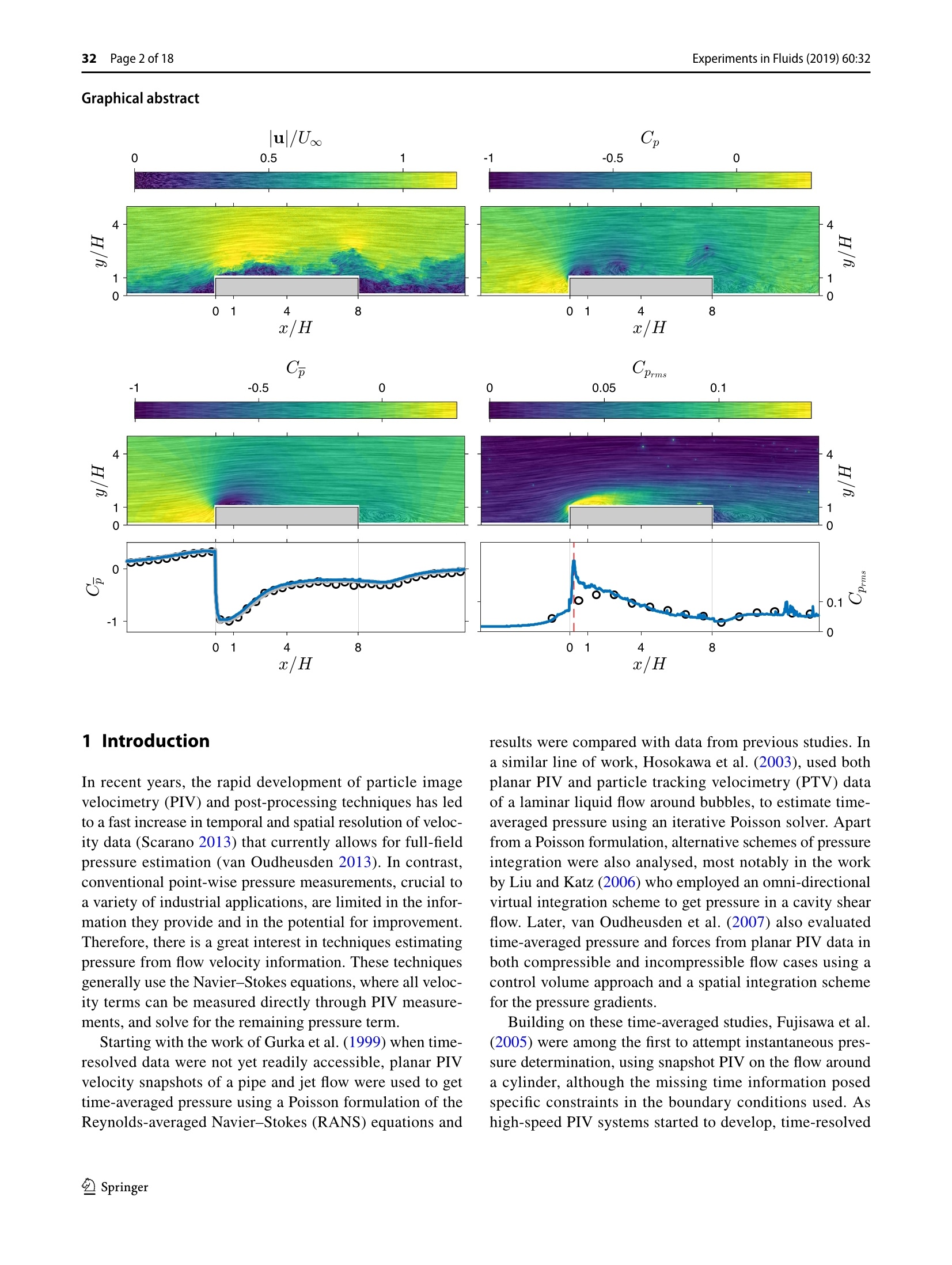
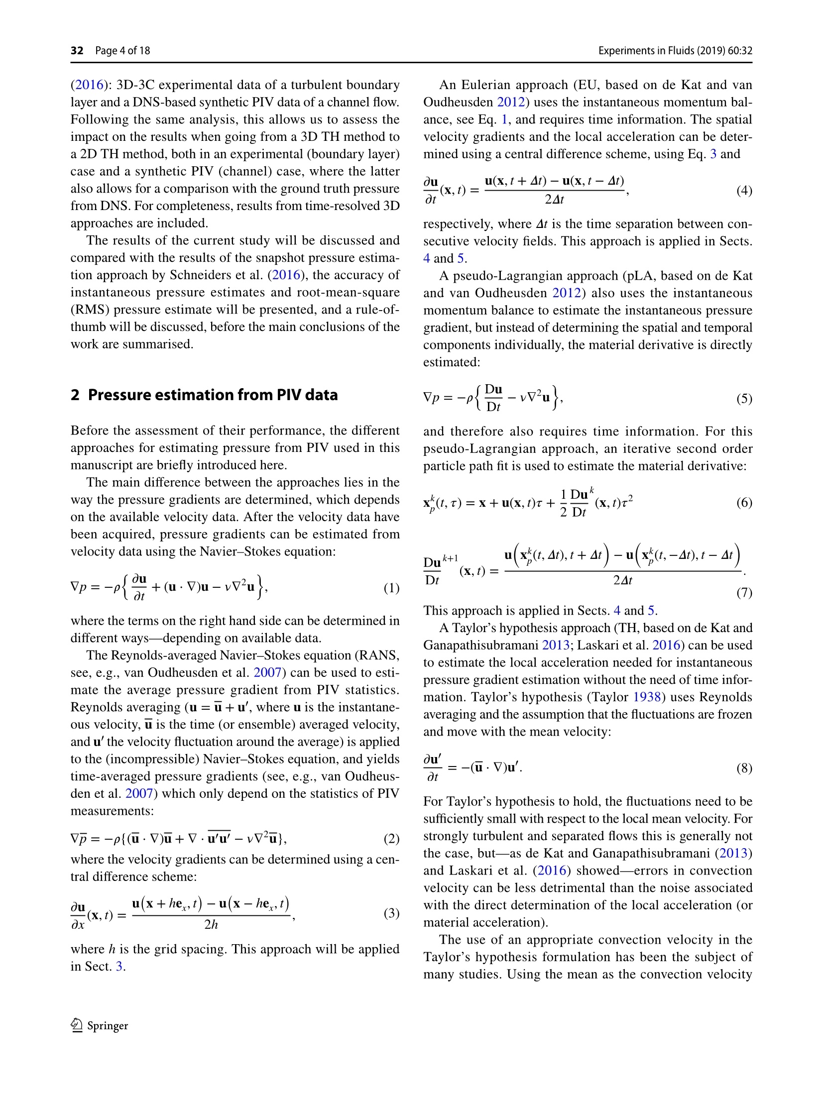
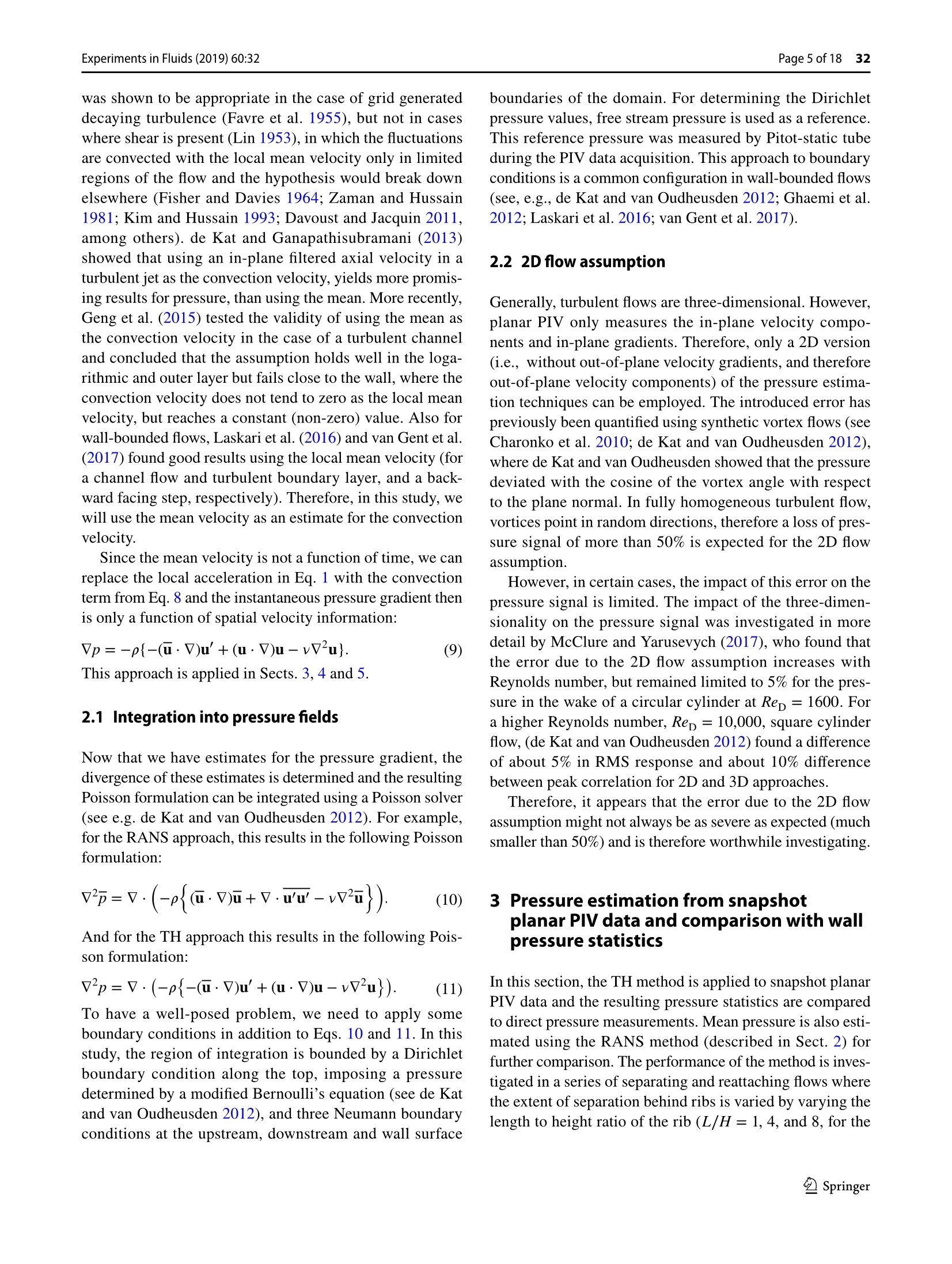
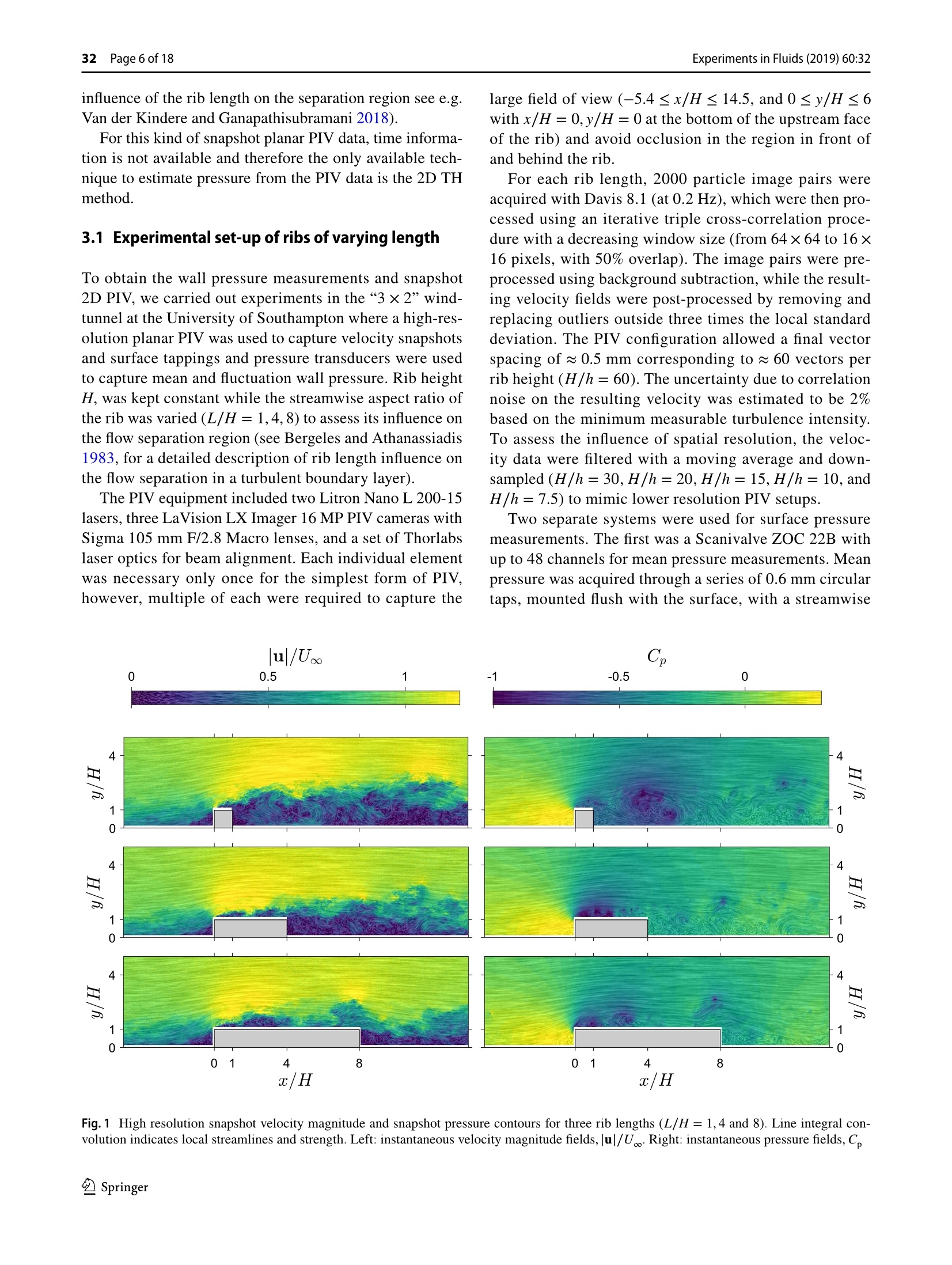
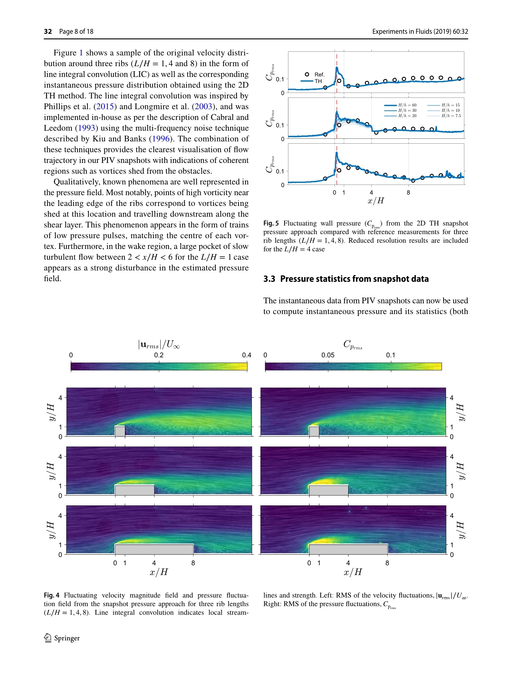
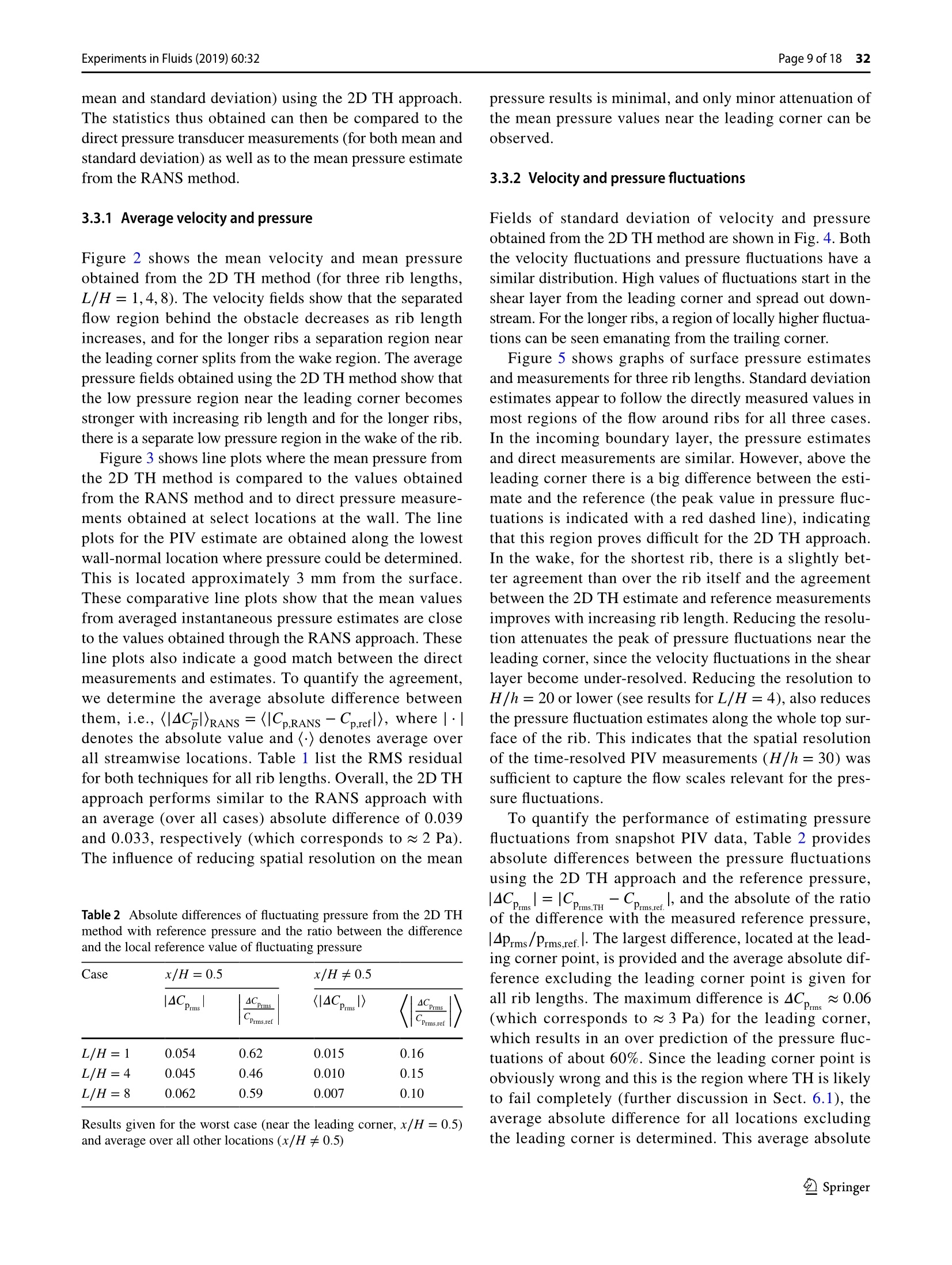
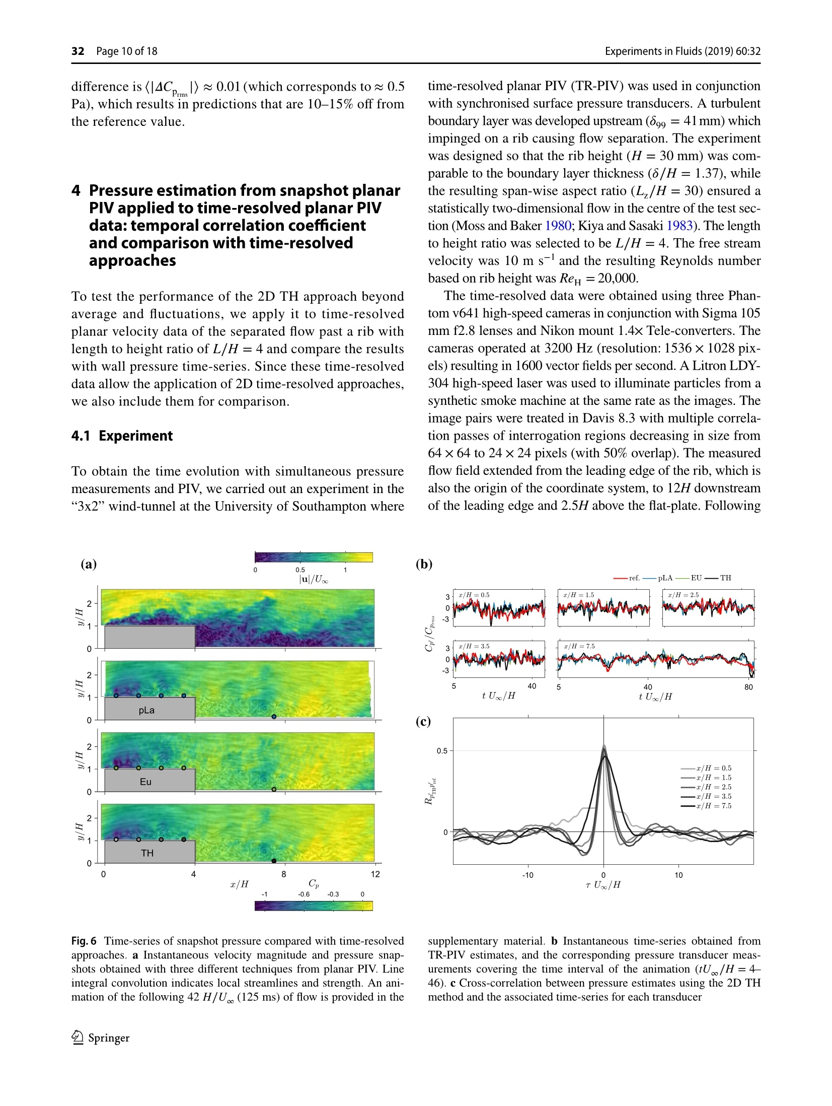
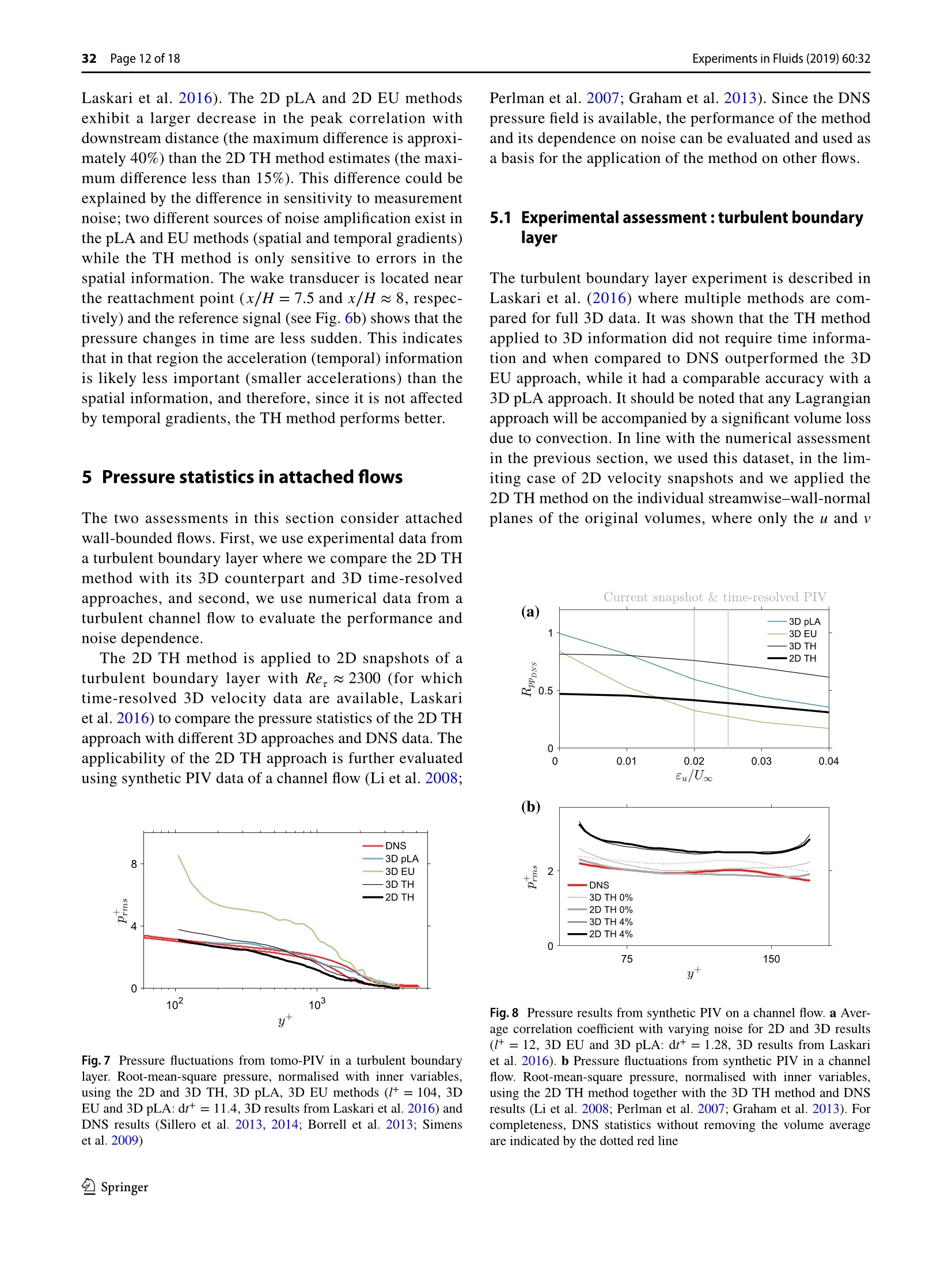
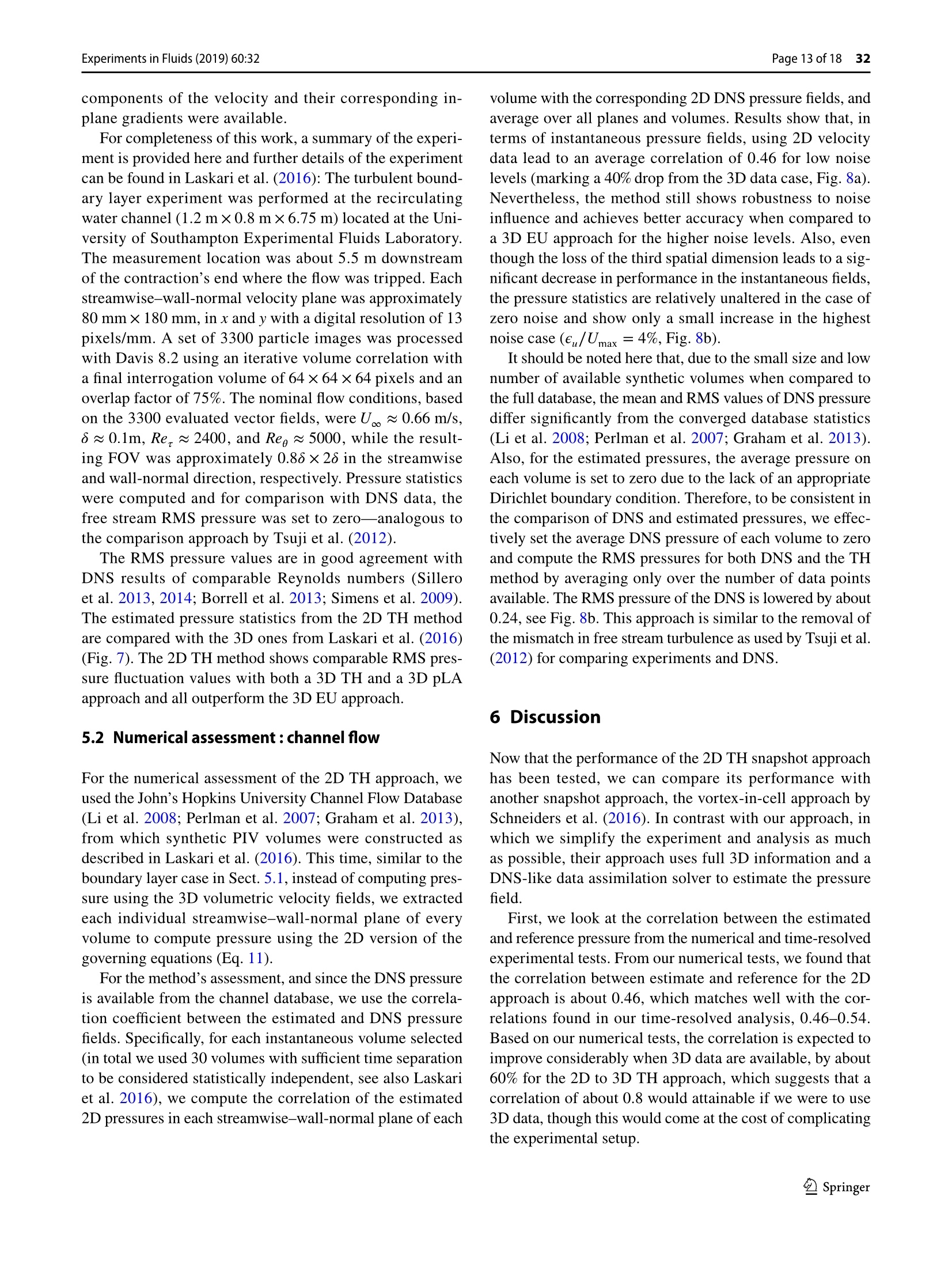
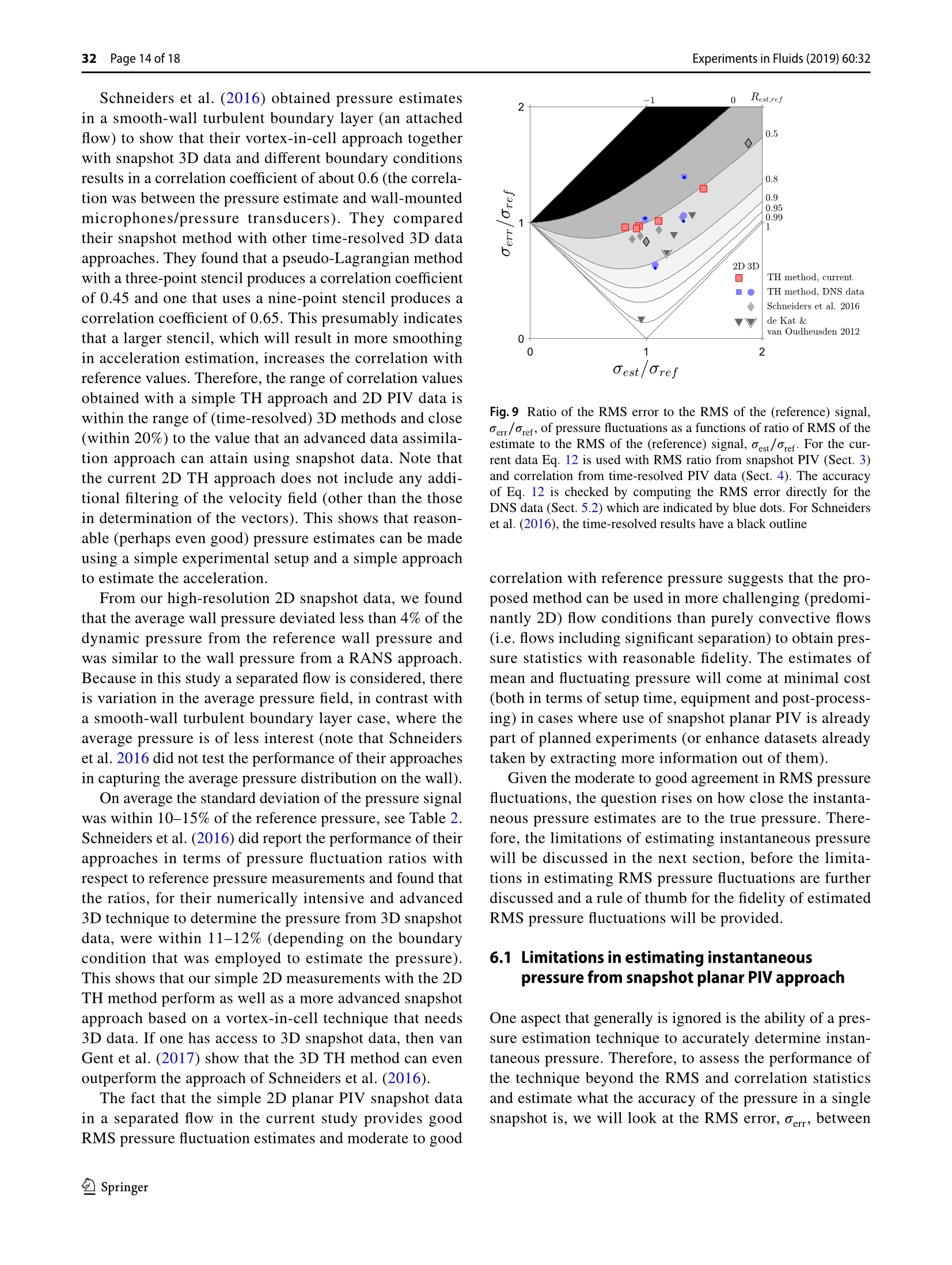
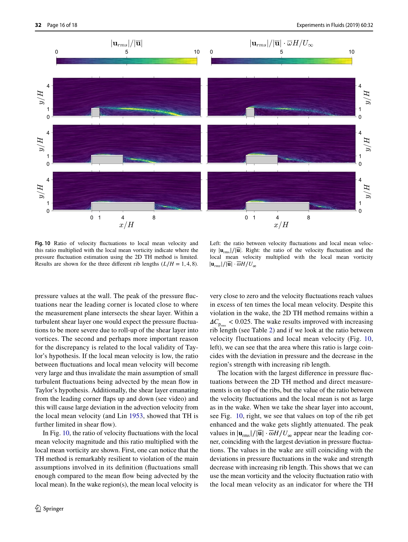
Experiments in Fluids (2019) 60:32https://doi.org/10.1007/s00348-019-2678-5 32 Page 2 of 18Experiments in Fluids (2019) 60:32 RESEARCH ARTICLE Pressure from 2D snapshot PIV J. W. Van der Kinderel. A. Laskari12. B. Ganapathisubramanil·R. de Kat( Received: 20 March 2018 / Revised: 20 December 2018 /Accepted: 3 January 2019 / Published online: 25 January 2019@ The Author(s) 2019 Abstract In this study, we quantify the accuracy of a simple pressure estimation method from 2D snapshot PIV in attached andseparated flows. Particle image velocimetry (PIV) offers the possibility to acquire a field of pressure instead of point meas-urements. Multiple methods may be used to obtain pressure from PIV measurements, however, the current state-of-the-artrequires expensive equipment and data processing. As an alternative, we aim to quantify the efficacy ofestimating instan-taneous pressure from snapshot (non-time resolved) two-dimensional planar PIV (the simplest type of PIV available). Tomake up for the loss oftemporal information, we rely on Taylor’s hypothesis (TH) to replace temporal information withspatial gradients. Application of our approach to high-resolution 2D velocity data of a turbulent boundary layer flow overribs shows moderate to good agreement with reference pressure measurements in average and fluctuations. To assess theperformance of the 2D TH method beyond average and fluctuation statistics, we acquired a time-resolved measurement ofthe same flow and determined temporal correlation values of the pressure from our method with reference measurements.Overall, the correlation attains good values for all measured locations. For comparison, we also applied two time-resolvedapproaches, which attained values of correlation similar to our approach. The performance of the 2D TH method is furtherassessed on 3D time-resolved velocity data for a turbulent boundary layer and compared with 3D methods. The root-mean-square (RMS) pressure fluctuations of the 2D TH, 3D TH and 3D pseudo-Lagrangian methods closely follow the pressurefluctuation distribution from DNS. These observations on the RMS pressure estimates are further supported by similaranalysis on synthetic PIV data (based on DNS) of a turbulent channel flow. The values of spatial correlation between the 2DTH method and the DNS pressure fields in this case, are similar to the temporal correlations achieved in the turbulent flowover the ribs. Finally, we discuss the accuracy of instantaneous pressure estimates and provide a rule of thumb to determineregions where the pressure fluctuation estimate from the 2D TH methods is likely to fail. Electronic supplementary material The online version of thisarticle (https://doi.org/10.1007/s00348-019-2678-5) containssupplementary material, which is available to authorized users. 区R. de Katr.de-kat@soton.ac.uk Department of Aeronautics and Astronautics, Universityof Southampton, Southampton SO17 1BJ, UK 2 Present Address: GALCIT. California Instituteof Technology, Pasadena, CA 91125, USA Graphical abstract 1 Introduction In recent years, the rapid development of particle imagevelocimetry (PIV) and post-processing techniques has ledto a fast increase in temporal and spatial resolution of veloc-ity data (Scarano 2013) that currently allows for full-fieldpressure estimation (van Oudheusden 2013). In contrast,conventional point-wise pressure measurements, crucial toa variety of industrial applications, are limited in the infor-mation they provide and in the potential for improvement.Therefore, there is a great interest in techniques estimatingpressure from flow velocity information. These techniquesgenerally use the Navier-Stokes equations, where all veloc-ity terms can be measured directly through PIV measure-ments, and solve for the remaining pressure term. Starting with the work of Gurka et al. (1999) when time-resolved data were not yet readily accessible, planar PIVvelocity snapshots of a pipe and jet flow were used to gettime-averaged pressure using a Poisson formulation of theReynolds-averaged Navier-Stokes (RANS) equations and results were compared with data from previous studies. Ina similar line of work, Hosokawa et al. (2003), used bothplanar PIV and particle tracking velocimetry (PTV) dataof a laminar liquid flow around bubbles, to estimate time-averaged pressure using an iterative Poisson solver. Apartfrom a Poisson formulation, alternative schemes of pressureintegration were also analysed, most notably in the workby Liu and Katz (2006) who employed an omni-directionalvirtual integration scheme to get pressure in a cavity shearflow. Later, van Oudheusden et al. (2007) also evaluatedtime-averaged pressure and forces from planar PIV data inboth compressible and incompressible flow cases using acontrol volume approach and a spatial integration schemefor the pressure gradients. Building on these time-averaged studies, Fujisawa et al.(2005) were among the first to attempt instantaneous pres-sure determination, using snapshot PIV on the flow arounda cylinder, although the missing time information posedspecific constraints in the boundary conditions used. Ashigh-speed PIV systems started to develop, time-resolved velocity information became available and several studies oninstantaneous pressure determination subsequently emerged(Liu and Katz 2006; Murai et al. 2007;de Kat et al. 2008),effectively shifting the attention towards evaluation methodsfor the material acceleration term. In that context both Eule-rian and Lagrangian approaches for the computation of theacceleration term were assessed in various flow scenarios.often with contradicting results (see Jakobsen et al. 1997;Charonko et al. 2010; Violato et al. 2011; de Kat and vanOudheusden 2012; Ghaemi et al. 2012, among others). AnEulerian approach was found to better match experimentalresults in the case of surface waves (Jakobsen et al. 1997),while a Lagrangian method was shown to be limited due topoor particle tracking and exhibited a small bias leading toa systematic error in pressure estimation. These results weresupported by de Kat and van Oudheusden (2012) who attrib-uted the limitations of a pseudo-Lagrangian technique—pseudo, because fluid parcel paths are estimated from thevelocity data instead of actually tracking a fluid parcel ortracer particle-due to the structures’turnover time, tobe more severe than the ones for an Eulerian approach. Incontrast to this, works from both Violato et al. (2011) andGhaemi et al. (2012) showed that a pseudo-Lagrangianapproach managed a lower precision error and was less sen-sitive to noise in comparison with an Eulerian method. However, new techniques that allow for accurate fullyLagrangian particle tracking have recently been developedand show great promise in improving material accelerationmeasurements (and therefore pressure estimation).Mostnotably, Schroder et al. (2015), and Schanz et al. (2016)presented a ‘Shake the Box'algorithm, which uses volumet-ric time-resolved particle images and reconstructs particletrajectories using previous time steps to predict future par-ticle positions and corrects accordingly using image match-ing. Such particle tracking methods provide highly accuratematerial acceleration estimations, significantly improvingpressure reconstruction when compared to methods that usePIV velocity information, which is known to suffer fromaveraging effects of the cross-correlation process involved(see van Gent et al. 2017, for a detailed comparison onpressure estimation using different PIV and PTV basedapproaches). These developments show that in a scientific context, pro-gress on pressure estimation techniques is oriented towardsstate-of-the-art equipment and complex computationalalgorithms. However,for some applications (e.g. indus-trial measurements), minimisation of cost, complexity andprocessing time is critical, and often balanced against theaccuracy of the technique. Therefore, to allow an informedchoice in this balance, it is valuable to quantify how lossof information (either in terms of time or space) affects theaccuracy of pressure estimation methods, so that a balancebetween cost and performance can be found for different applications (see, e.g., McClure and Yarusevych 2017, foran exposition of 2D vs 3D measurements, time and spatialresolution in turbulent wake flows). In a bid to simplify the measurement equipment needed,one could use models to remove the requirement to capturea time-series altogether. Schneiders et al. (2016) proposeda method based on the vorticity transport equation to esti-mate instantaneous pressure from 3D velocity snapshotswhen time information is not available, however, this is acomplex procedure which still requires (complicated) volu-metric-PIV/PTV measurement. A different approach is to use Taylor’s hypothesis (TH) tofill in the missing spatial information (de Kat and Ganapa-thisubramani 2013) or time information (de Kat and Gana-pathisubramani 2013; Laskari et al. 2016). The use of THwas assessed in the case of time-resolved 3C-planar data(de Kat and Ganapathisubramani 2013) and 3C-volumetricsnapshots (Laskari et al.2016) and reliable pressure esti-mates were found for both, missing spatial and temporalinformation respectively, while the TH method also provedto be the most robust approach with respect to noise and gridresolution (Laskari et al.2016). However, these studies still require either time-resolvedstereo or snapshot tomographic PIV to acquire 3C velocitydata. Our goal in the present work is to assess the perfor-mance of the TH approach in the simplest possible setup,snapshot 2D PIV. We assess the performance of pressure determinationwith the TH method using 2D velocity snapshots in bothseparated and wall-bounded flows and compare its perfor-mance versus reference measures.Additionally—measure-ment data allowing—we provide comparisons with alter-native techniques. We start with describing the differentapproaches used in this study,before applying them to fourdifferent data sets, with the main goal to assess differentperformance aspects of the 2D TH method. First, we showcase pressure estimation using high-reso-lution 2D snapshot measurements, where no other techniqueapplies, and consider ribs of different lengths which allow toassess the influence of size (and strength) of the separationregion (Van der Kindere and Ganapathisubramani 2018).The resulting estimated pressures are compared statisticallywith wall pressure measurements. Second, because statistical measures can obscure and bal-ance noise sources, we use 2D time-resolved data to deter-mine the temporal cross-correlation of the pressure signalwith wall pressure measurements, which provides informa-tion on how closely the estimated and measured time-seriesmatch in time. These time-resolved data also allow for 2Dtime-resolved pressure estimation approaches, therefore, forcompleteness, their results are included. Third, because turbulent flows are inherently 3D we willapply the 2D TH method to the data from Laskari et al. (2016): 3D-3C experimental data of a turbulent boundarylayer and a DNS-based synthetic PIV data of a channel flow.Following the same analysis, this allows us to assess theimpact on the results when going from a 3D TH method toa 2D TH method, both in an experimental (boundary layer)case and a synthetic PIV (channel) case, where the latteralso allows for a comparison with the ground truth pressurefrom DNS. For completeness, results from time-resolved 3Dapproaches are included. The results of the current study will be discussed andcompared with the results of the snapshot pressure estima-tion approach by Schneiders et al. (2016), the accuracy ofinstantaneous pressure estimates and root-mean-square(RMS) pressure estimate will be presented, and a rule-of-thumb will be discussed, before the main conclusions of thework are summarised. 2 Pressure estimation from PIV data Before the assessment of their performance, the differentapproaches for estimating pressure from PIV used in thismanuscript are briefly introduced here. The main difference between the approaches lies in theway the pressure gradients are determined,which dependson the available velocity data. After the velocity data havebeen acquired, pressure gradients can be estimated fromvelocity data using the Navier-Stokes equation: where the terms on the right hand side can be determined indifferent ways-depending on available data. The Reynolds-averaged Navier-Stokes equation (RANS,see, e.g., van Oudheusden et al.2007) can be used to esti-mate the average pressure gradient from PIV statistics.Reynolds averaging (u=u+u’, where u is the instantane-ous velocity, u is the time (or ensemble) averaged velocity,and u’ the velocity fluctuation around the average) is appliedto the (incompressible) Navier-Stokes equation, and yieldstime-averaged pressure gradients (see, e.g., van Oudheus-den et al. 2007) which only depend on the statistics of PIVmeasurements: where the velocity gradients can be determined using a cen-tral difference scheme: where h is the grid spacing. This approach will be appliedin Sect. 3. An Eulerian approach (EU, based on de Kat and vanOudheusden 2012) uses the instantaneous momentum bal-ance, see Eq. 1, and requires time information. The spatialvelocity gradients and the local acceleration can be deter-mined using a central difference scheme, using Eq. 3 and respectively, where At is the time separation between con-secutive velocity fields. This approach is applied in Sects.4 and 5. A pseudo-Lagrangian approach (pLA, based on de Katand van Oudheusden 2012) also uses the instantaneousmomentum balance to estimate the instantaneous pressuregradient, but instead of determining the spatial and temporalcomponents individually, the material derivative is directlyestimated: and therefore also requires time information. For thispseudo-Lagrangian approach, an iterative second orderparticle path fit is used to estimate the material derivative: This approach is applied in Sects. 4 and 5. A Taylor’s hypothesis approach (TH, based on de Kat andGanapathisubramani 2013; Laskari et al. 2016) can be usedto estimate the local acceleration needed for instantaneouspressure gradient estimation without the need of time infor-mation. Taylor’s hypothesis (Taylor 1938) uses Reynoldsaveraging and the assumption that the fluctuations are frozenand move with the mean velocity: For Taylor’s hypothesis to hold, the fluctuations need to besufficiently small with respect to the local mean velocity. Forstrongly turbulent and separated flows this is generally notthe case, but-as de Kat and Ganapathisubramani (2013)and Laskari et al. (2016) showed-errors in convectionvelocity can be less detrimental than the noise associatedwith the direct determination of the local acceleration (ormaterial acceleration). The use of an appropriate convection velocity in theTaylor’s hypothesis formulation has been the subject ofmany studies. Using the mean as the convection velocity was shown to be appropriate in the case of grid generateddecaying turbulence (Favre et al. 1955), but not in caseswhere shear is present (Lin 1953), in which the fluctuationsare convected with the local mean velocity only in limitedregions of the flow and the hypothesis would break downelsewhere (Fisher and Davies 1964; Zaman and Hussain1981; Kim and Hussain 1993; Davoust and Jacquin 2011,among others). de Kat and Ganapathisubramani (2013)showed that using an in-plane filtered axial velocity in aturbulent jet as the convection velocity, yields more promis-ing results for pressure, than using the mean. More recently,Geng et al. (2015) tested the validity of using the mean asthe convection velocity in the case of a turbulent channeland concluded that the assumption holds well in the loga-rithmic and outer layer but fails close to the wall, where theconvection velocity does not tend to zero as the local meanvelocity, but reaches a constant (non-zero) value. Also forwall-bounded flows, Laskari et al. (2016) and van Gent et al.(2017) found good results using the local mean velocity (fora channel flow and turbulent boundary layer, and a back-ward facing step, respectively). Therefore, in this study, wewill use the mean velocity as an estimate for the convectionvelocity. Since the mean velocity is not a function of time, we canreplace the local acceleration in Eq. 1 with the convectionterm from Eq. 8 and the instantaneous pressure gradient thenis only a function of spatial velocity information: This approach is applied in Sects. 3, 4 and 5. 2.1 Integration into pressure fields Now that we have estimates for the pressure gradient, thedivergence of these estimates is determined and the resultingPoisson formulation can be integrated using a Poisson solver(see e.g. de Kat and van Oudheusden 2012). For example,for the RANS approach, this results in the following Poissonformulation: And for the TH approach this results in the following Pois-son formulation: To have a well-posed problem, we need to apply someboundary conditions in addition to Eqs. 10 and 11. In thisstudy, the region of integration is bounded by a Dirichletboundary condition along the top, imposing a pressuredetermined by a modified Bernoulli’s equation (see de Katand van Oudheusden 2012), and three Neumann boundaryconditions at the upstream, downstream and wall surface boundaries of the domain. For determining the Dirichletpressure values, free stream pressure is used as a reference.This reference pressure was measured by Pitot-static tubeduring the PIV data acquisition. This approach to boundaryconditions is a common configuration in wall-bounded flows(see, e.g., de Kat and van Oudheusden 2012; Ghaemi et al.2012; Laskari et a. 2016; van Gent et al.2017). 2.2 2D flow assumption Generally, turbulent flows are three-dimensional. However,planar PIV only measures the in-plane velocity compo-nents and in-plane gradients. Therefore, only a 2D version(i.e., without out-of-plane velocity gradients, and thereforeout-of-plane velocity components) of the pressure estima-tion techniques can be employed. The introduced error haspreviously been quantified using synthetic vortex flows (seeCharonko et al. 2010; de Kat and van Oudheusden 2012),where de Kat and van Oudheusden showed that the pressuredeviated with the cosine of the vortex angle with respectto the plane normal. In fully homogeneous turbulent flow,vortices point in random directions, therefore a loss of pres-sure signal of more than 50% is expected for the 2D flowassumption. However, in certain cases, the impact of this error on thepressure signal is limited. The impact of the three-dimen-sionality on the pressure signal was investigated in moredetail by McClure and Yarusevych (2017), who found thatthe error due to the 2D flow assumption increases withReynolds number, but remained limited to 5% for the pres-sure in the wake of a circular cylinder at Rep=1600. Fora higher Reynolds number, Rep=10,000, square cylinderflow, (de Kat and van Oudheusden 2012) found a differenceof about 5% in RMS response and about 10% differencebetween peak correlation for 2D and 3D approaches. Therefore, it appears that the error due to the 2D flowassumption might not always be as severe as expected (muchsmaller than 50%) and is therefore worthwhile investigating. 3 Pressure estimation from snapshotplanar PIV data and comparison with wallpressure statistics In this section, the TH method is applied to snapshot planarPIV data and the resulting pressure statistics are comparedto direct pressure measurements. Mean pressure is also esti-mated using the RANS method (described in Sect. 2) forfurther comparison. The performance of the method is inves-tigated in a series of separating and reattaching flows wherethe extent of separation behind ribs is varied by varying thelength to height ratio of the rib (L/H=1, 4, and 8, for the influence of the rib length on the separation region see e.g.Van der Kindere and Ganapathisubramani 2018). For this kind of snapshot planar PIV data, time informa-tion is not available and therefore the only available tech-nique to estimate pressure from the PIV data is the 2D THmethod. 3.1 Experimental set-up of ribs of varying length To obtain the wall pressure measurements and snapshot2D PIV, we carried out experiments in the “3×2”wind-tunnel at the University of Southampton where a high-res-olution planar PIV was used to capture velocity snapshotsand surface tappings and pressure transducers were usedto capture mean and fluctuation wall pressure. Rib heightH, was kept constant while the streamwise aspect ratio ofthe rib was varied (L/H=1,4,8) to assess its influence onthe flow separation region (see Bergeles and Athanassiadis1983, for a detailed description of rib length influence onthe flow separation in a turbulent boundary layer). The PIV equipment included two Litron Nano L 200-15lasers, three La Vision LX Imager 16 MP PIV cameras withSigma 105 mm F/2.8 Macro lenses, and a set of Thorlabslaser optics for beam alignment. Each individual elementwas necessary only once for the simplest form of PIV,however, multiple of each were required to capture the Fig.1 High resolution snapshot velocity magnitude and snapshot pressure contours for three rib lengths (L/H=1,4 and 8). Line integral con-volution indicates local streamlines and strength. Left: instantaneous velocity magnitude fields,|u|/U.Right: instantaneous pressure fields, C, large field of view (-5.4≤x/H≤14.5, and0≤y/H≤6with x/H=0,y/H=0 at the bottom of the upstream faceof the rib) and avoid occlusion in the region in front ofand behind the rib. For each rib length, 2000 particle image pairs wereacquired with Davis 8.1 (at 0.2 Hz), which were then pro-cessed using an iterative triple cross-correlation proce-dure with a decreasing window size (from 64× 64 to 16 ×16 pixels, with 50% overlap). The image pairs were pre-processed using background subtraction, while the result-ing velocity fields were post-processed by removing andreplacing outliers outside three times the local standarddeviation. The PIV configuration allowed a final vectorspacing of ~ 0.5 mm corresponding to ~ 60 vectors perrib height (H/h=60). The uncertainty due to correlationnoise on the resulting velocity was estimated to be 2%based on the minimum measurable turbulence intensity.To assess the influence of spatial resolution, the veloc-ity data were filtered with a moving average and down-sampled (H/h=30,H/h=20,H/h=15,H/h=10, andH/h=7.5) to mimic lower resolution PIV setups. Two separate systems were used for surface pressuremeasurements. The first was a Scanivalve ZOC 22B withup to 48 channels for mean pressure measurements. Meanpressure was acquired through a series of 0.6 mmcirculartaps, mounted flush with the surface, with a streamwise 0.5 x/H Fig.2 Average velocity magnitude field and pressure field fromthe 2D TH snapshot pressure approach for three rib lengths(L/H=1,4,8). Line integral convolution indicates local streamlines Fig.3 Average wall pressure using the 2D TH and RANS approachcompared with reference measurements for three rib lengths(L/H=1,4,8), C,. Reduced resolution results are included for theL/H=4 case spacing of 0.5H, the first one located at x/H=-8.25.Thetaps were aligned in the streamwise direction with the PIVmeasurement plane. The second system was necessary forpressure fluctuations. It consisted of two Endevco 8507C-2pressure transducers and a third Endevco 8510-1B con-nected to the surface by a 0.8 mm wide, 2 mm long hole.The 8507C-2 transducers measured pressure fluctuations |/U.. C, 0 -1 -0.5 0 c/H and strength. Left: average velocity magnitude field,u|/U.. Right:average pressure field,c, Table 1 Average of absolute differences of mean pressure for RANSand 2D TH with reference pressure Case (I4C,I)RANS (I4C,I)TH L/H=1 0.043 0.047 L/H=4 0.024 0.029 L/H=8 0.033 0.042 from x/H=-1 to 14.5, whereas the 8510-1B transducerwas placed far upstream to capture uncorrelated pressuresignal that is necessary for optimal noise cancellation asper Naguib et al. (1996). In total, the transducers weresampled four times for 30 s at the rate of 25.6 kHz. Thesignal from each transducer was filtered first through opti-mal noise removal filter and subsequently low-pass filteredat 1280 Hz. 3.2 Instantaneous snapshot pressure results In keeping with a simple PIV configuration, only uncorre-lated snapshot PIV measurements were obtained in this setof experiments. This allows the use of the 2D TH methodto obtain instantaneous pressure from the snapshot data andsubsequently, pressure statistics. Figure 1 shows a sample of the original velocity distri-bution around three ribs (L/H=1,4 and 8) in the form ofline integral convolution (LIC) as well as the correspondinginstantaneous pressure distribution obtained using the 2DTH method. The line integral convolution was inspired byPhillips et al. (2015) and Longmire et al. (2003), and wasimplemented in-house as per the description of Cabral andLeedom (1993) using the multi-frequency noise techniquedescribed by Kiu and Banks (1996). The combination ofthese techniques provides the clearest visualisation of flowtrajectory in our PIV snapshots with indications of coherentregions such as vortices shed from the obstacles. Qualitatively, known phenomena are well represented inthe pressure field. Most notably, points of high vorticity nearthe leading edge of the ribs correspond to vortices beingshed at this location and travelling downstream along theshear layer. This phenomenon appears in the form of trainsof low pressure pulses, matching the centre of each vor-tex. Furthermore, in the wake region, a large pocket of slowturbulent flow between 2 ≈ 0.01 (which corresponds to ≈ 0.5Pa), which results in predictions that are 10-15% off fromthe reference value. 4 Pressure estimation from snapshot planarPIV applied to time-resolved planar PIVdata: temporal correlation coefficientand comparison with time-resolvedapproaches To test the performance of the 2D TH approach beyondaverage and fluctuations, we apply it to time-resolvedplanar velocity data of the separated flow past a rib withlength to height ratio of L/H= 4 and compare the resultswith wall pressure time-series. Since these time-resolveddata allow the application of 2D time-resolved approaches,we also include them for comparison. 4.1 Experiment To obtain the time evolution with simultaneous pressuremeasurements and PIV, we carried out an experiment in the“3x2”wind-tunnel at the University of Southampton where Fig.6 Time-series of snapshot pressure compared with time-resolvedapproaches. a Instantaneous velocity magnitude and pressure snap-shots obtained with three different techniques from planar PIV. Lineintegral convolution indicates local streamlines and strength. An ani-mation of the following 42 H/U,(125 ms) of flow is provided in the time-resolved planar PIV (TR-PIV) was used in conjunctionwith synchronised surface pressure transducers. A turbulentboundary layer was developed upstream (89g=41mm) whichimpinged on a rib causing flow separation. The experimentwas designed so that the rib height (H=30 mm) was com-parable to the boundary layer thickness (8/H=1.37), whilethe resulting span-wise aspect ratio (L/H=30) ensured astatistically two-dimensional flow in the centre of the test sec-tion (Moss and Baker 1980; Kiya and Sasaki 1983). The lengthto height ratio was selected to be L/H=4. The free streamvelocity was 10 m s-l and the resulting Reynolds numberbased on rib height was Ren=20,000. The time-resolved data were obtained using three Phan-tom v641 high-speed cameras in conjunction with Sigma 105mm f2.8 lenses and Nikon mount 1.4× Tele-converters. Thecameras operated at 3200 Hz (resolution:1536×1028 pix-els) resulting in 1600 vector fields per second. A Litron LDY-304 high-speed laser was used to illuminate particles from asynthetic smoke machine at the same rate as the images. Theimage pairlsi rwse rWe treated in Davis 8.3 with multiple correla-tion passes of interrogation regions decreasing in size from64×64 to 24×24 pixels (with 50% overlap). The measuredflow field extended from the leading edge of the rib, which isalso the origin of the coordinate system, to 12H downstreamofthe leading edge and 2.5H above the flat-plate. Following (b) supplementary material. b Instantaneous time-series obtained fromTR-PIV estimates, and the corresponding pressure transducer meas-urements covering the time interval of the animation (tU/H= 4-46).c Cross-correlation between pressure estimates using the 2D THmethod and the associated time-series for each transducer Sciacchitano and Wieneke (2016), the uncertainty on thevelocity fluctuations was approximately 2.5%. The final vec-tor spacing was approximately 1 mm corresponding to ~ 30vectors per rib height (H/h=30), which was sufficient toestimate the correct level of pressure fluctuations (see previ-ous section). At the same time as the velocity measurements, fiveEndevco 8507C-2 pressure transducers were used to recordsurface pressure fluctuations at x/H=0.5,1.5,2.5,3.5, and7.5. To ensure synchronisation, the PIV trigger signal wasalso acquired by the pressure measurement system. A sixthEndevco 8510-1B was placed far upstream to acquire anuncorrelated pressure signal that could then be used for opti-mal noise cancellation as described by Naguib et al. (1996).These transducers were sampled at an acquisition rate of25.6 kHz. The data were de-noised and low-pass filtered at1280 Hz. 4.2 Application of the 2D TH method to 2Dmeasurements and comparison with 2Dtime-resolved approaches To further establish the performance of the 2D TH methodwith planar measurements, time-series of estimated pressureare compared with wall pressure measurements. In addi-tion, results of two time-resolved approaches are includedfor comparison. Figure 6 shows an example of a velocitysnapshot and resulting pressure estimates, time-series ofwall pressure for five locations for the different techniquesand cross-correlation between wall pressure and the pressurefrom the 2D TH method. Figure 6a contains sample snapshots of the instantaneouspressure estimate—using the three different methods: 2DEU, 2D pLA and 2D TH—around the rib. The evolution ofstreamlines is visualised with a line integral convolution asbefore. A video of the evolution of the velocity and pres-sure fields starting from the snapshots in Fig.6a (using antechnique similar to the dynamic LIC technique describedby Sundquist 2003) is provided in the supplementary mate-rial. The three methods appear to produce similar resultsbehind the leading edge, where shear layer roll-up and vortexshedding occurs. The range of pressure computed within the Table 3 Table containing the peak correlation coefficient betweenestimated and measured surface pressure Location,x/H= 0.5 1.5 2.5 3.5 7.5 2D pLA 0.53 0.55 0.52 0.48 0.34 2DEU 0.57 0.57 0.52 0.48 0.34 2D TH 0.52 0.54 0.50 0.51 0.46 The estimates come from the nearest point to the surface with validdata, this may be several vectors above the surface due to reflections domain is comparable across all methods. However, ThepLA and EU methods tend to introduce more fluctuationstowards the edges of the domain of integration. In addi-tion, the Eulerian method shows what seems to be a morenoisy result throughout the integration domain. This is nota physical feature of the flow as highlighted in the follow-ing section. The concurrent surface pressure fluctuation measure-ments are used to provide a reference for the pressureestimates described above. To compare these results, apressure time-series is extracted from the nearest validpoint to the pressure transducer. The measured and esti-mated time-series are synchronised in time therefore directcomparison is possible. Figure 6b depicts samples of thetime-series obtained through direct measurements, and theestimates from 2D pLA, 2D EU and 2D TH methods for alltransducer locations (as indicated in Fig. 6a). For the loca-tions on top of the rib (x/H=0.5, 1.5,2.5 and 3.5), theestimates appear to follow the reference signal quite wellwith no significant differences between the methods. Inthe wake region, the estimates follow the reference signal,but there is more differentiation between the methods. Athigher frequencies, peaks in the pressure estimates from2D EU and 2D pLA are present that are not mirrored inthe reference signal. The 2D TH method seems to producea smoother signal which follows the general trend of thetwo other estimates and also appears to follow the refer-ence signal better. To quantify the performance of the different approaches,cross-correlation coefficients between estimates and thedirect measurements are determined. Figure 6c shows thecross-correlation R, computed between the signal fromfive pressure transducers and the nearest pressure time-series estimated using the 2D TH method (location arealso indicated in Fig. 6a). The figure shows the peak cor-relation is at zero time lag indicating that there is no phasedifference between measured and estimated pressure atthese locations. Figure 6c also shows that the peak correla-tion value decreases with increasing streamwise location.The same procedure was repeated for the two other estima-tion methods and no measurable time-delay was foundbetween signals. The other methods also decrease in peakcorrelation value with downstream distance. The peak cross-correlation coefficient for all streamwiselocations and all three methods is reported in Table 3. The2D TH method shows a maximum R,,of 0.54 along thetop surface of the obstacle, and 0.46 in the wake region.The highest correlation value is comparable to the othertwo methods. The comparable accuracy could be due tothe fact that the TH method is more robust to measurementnoise compared to the Eulerian and pseudo-Lagrangianmethods (see de Kat and Ganapathisubramani 2013; Laskari et al. 2016). The 2D pLA and 2D EU methodsexhibit a larger decrease in the peak correlation withdownstream distance (the maximum difference is approxi-mately 40%) than the 2D TH method estimates (the maxi-mum difference less than 15%). This difference could beexplained by the difference in sensitivity to measurementnoise; two different sources of noise amplification exist inthe pLA and EU methods (spatial and temporal gradients)while the TH method is only sensitive to errors in thespatial information. The wake transducer is located nearthe reattachment point (x/H= 7.5 and x/H~8, respec-tively) and the reference signal (see Fig.6b) shows that thepressure changes in time are less sudden. This indicatesthat in that region the acceleration (temporal) informationis likely less important (smaller accelerations) than thespatial information, and therefore, since it is not affectedby temporal gradients, the TH method performs better. 5 Pressure statistics in attached flows The two assessments in this section consider attachedwall-bounded flows. First, we use experimental data froma turbulent boundary layer where we compare the 2D THmethod with its 3D counterpart and 3D time-resolvedapproaches, and second, we use numerical data from aturbulent channel flow to evaluate the performance andnoise dependence. The 2D TH method is applied to 2D snapshots of aturbulent boundary layer with Re≈2300 (for whichtime-resolved 3D velocity data are available, Laskariet al.2016) to compare the pressure statistics of the 2D THapproach with different 3D approaches and DNS data. Theapplicability of the 2D TH approach is further evaluatedusing synthetic PIV data of a channel flow (Li et al. 2008; Fig.7 Pressure fluctuations from tomo-PIV in a turbulent boundarylayer. Root-mean-square pressure, normalised with inner variables,using the 2D and 3D TH, 3D pLA, 3D EU methods (I+= 104, 3DEU and3D pLA: dt+=11.4,3D results from Laskari et al. 2016) andDNS results (Sillero et al. 2013, 2014; Borrell et al. 2013; Simenset al. 2009 Perlman et al. 2007; Graham et al. 2013). Since the DNSpressure field is available, the performance of the methodand its dependence on noise can be evaluated and used asa basis for the application of the method on other flows. 5.1 Experimental assessment :turbulent boundarylayer The turbulent boundary layer experiment is described inLaskari et al. (2016) where multiple methods are com-pared for full 3D data. It was shown that the TH methodapplied to 3D information did not require time informa-tion and when compared to DNS outperformed the 3DEU approach, while it had a comparable accuracy with a3D pLA approach. It should be noted that any Lagrangianapproach will be accompanied by a significant volume lossdue to convection. In line with the numerical assessmentin the previous section, we used this dataset, in the lim-iting case of 2D velocity snapshots and we applied the2D TH method on the individual streamwise-wall-normalplanes of the original volumes, where only the u and v Fig.8 Pressure results from synthetic PIV on a channel flow. a Aver-age correlation coefficient with varying noise for 2D and 3D results(I+=12, 3D EU and 3D pLA: dt+=1.28, 3D results from Laskariet al. 2016). b Pressure fluctuations from synthetic PIV in a channelflow. Root-mean-square pressure, normalised with inner variables,using the 2D TH method together with the 3D TH method and DNSresults (Li et al. 2008; Perlman et al. 2007; Graham et al. 2013). Forcompleteness, DNS statistics without removing the volume averageare indicated by the dotted red line components of the velocity and their corresponding in-plane gradients were available. For completeness of this work, a summary of the experi-ment is provided here and further details of the experimentcan be found in Laskari et al. (2016): The turbulent bound-ary layer experiment was performed at the recirculatingwater channel (1.2 m×0.8m×6.75 m) located at the Uni-versity of Southampton Experimental Fluids Laboratory.The measurement location was about 5.5 m downstreamof the contraction’s end where the flow was tripped. Eachstreamwise-wall-normal velocity plane was approximately80 mm×180 mm, in x and y with a digital resolution of 13pixels/mm. A set of 3300 particle images was processedwith Davis 8.2 using an iterative volume correlation witha final interrogation volume of 64×64×64 pixels and anoverlap factor of 75%. The nominal flow conditions, basedon the 3300 evaluated vector fields, were U~0.66 m/s,8~0.1m, Re,~ 2400, and Re ~5000, while the result-ing FOV was approximately 0.88×28 in the streamwiseand wall-normal direction, respectively. Pressure statisticswere computed and for comparison with DNS data, thefree stream RMS pressure was set to zero—analogous tothe comparison approach by Tsuji et al.(2012). The RMS pressure values are in good agreement withDNS results of comparable Reynolds numbers (Silleroet al. 2013, 2014; Borrell et al. 2013; Simens et al. 2009).The estimated pressure statistics from the 2D TH methodare compared with the 3D ones from Laskari et al. (2016)(Fig.7). The 2D TH method shows comparable RMS pres-sure fluctuation values with both a 3D TH and a 3D pLAapproach and all outperform the 3D EU approach. 5.2 Numerical assessment :channel flow For the numerical assessment of the 2D TH approach, weused the John’s Hopkins University Channel Flow Database(Li et al. 2008; Perlman et al. 2007; Graham et al. 2013),from which synthetic PIV volumes were constructed asdescribed in Laskari et al. (2016). This time, similar to theboundary layer case in Sect. 5.1, instead of computing pres-sure using the 3D volumetric velocity fields, we extractedeach individual streamwise-wall-normal plane of everyvolume to compute pressure using the 2D version of thegoverning equations (Eq. 11). For the method’s assessment, and since the DNS pressureis available from the channel database, we use the correla-tion coefficient between the estimated and DNS pressurefields. Specifically, for each instantaneous volume selected(in total we used 30 volumes with sufficient time separationto be considered statistically independent, see also Laskariet al. 2016), we compute the correlation of the estimated2D pressures in each streamwise-wall-normal plane of each volume with the corresponding 2D DNS pressure fields, andaverage over all planes and volumes. Results show that, interms of instantaneous pressure fields, using 2D velocitydata lead to an average correlation of 0.46 for low noiselevels (marking a 40% drop from the 3D data case, Fig.8a).Nevertheless, the method still shows robustness to noiseinfluence and achieves better accuracy when compared toa3D EU approach for the higher noise levels. Also, eventhough the loss of the third spatial dimension leads to a sig-nificant decrease in performance in the instantaneous fields,the pressure statistics are relatively unaltered in the case ofzero noise and show only a small increase in the highestnoise case (eu/Umax =4%,Fig.8b). It should be noted here that, due to the small size and lownumber of available synthetic volumes when compared tothe full database, the mean and RMS values of DNS pressurediffer significantly from the converged database statistics(Li et al. 2008; Perlman et al. 2007; Graham et al. 2013).Also, for the estimated pressures, the average pressure oneach volume is set to zero due to the lack of an appropriateDirichlet boundary condition. Therefore, to be consistent inthe comparison of DNS and estimated pressures, we effec-tively set the average DNS pressure of each volume to zeroand compute the RMS pressures for both DNS and the THmethod by averaging only over the number of data pointsavailable. The RMS pressure of the DNS is lowered by about0.24, see Fig. 8b. This approach is similar to the removal ofthe mismatch in free stream turbulence as used by Tsuji et al.(2012) for comparing experiments and DNS. 6 Discussion Now that the performance of the 2D TH snapshot approachhas been tested, we can compare its performance withanother snapshot approach, the vortex-in-cell approach bySchneiders et al.(2016). In contrast with our approach, inwhich we simplify the experiment and analysis as muchas possible, their approach uses full 3D information and aDNS-like data assimilation solver to estimate the pressurefield. First, we look at the correlation between the estimatedand reference pressure from the numerical and time-resolvedexperimental tests. From our numerical tests, we found thatthe correlation between estimate and reference for the 2Dapproach is about 0.46, which matches well with the cor-relations found in our time-resolved analysis, 0.46-0.54.Based on our numerical tests, the correlation is expected toimprove considerably when 3D data are available, by about60% for the 2D to 3D TH approach, which suggests that acorrelation of about 0.8 would attainable if we were to use3D data, though this would come at the cost of complicatingthe experimental setup. Schneiders et al. (2016) obtained pressure estimatesin a smooth-wall turbulent boundary layer (an attachedflow) to show that their vortex-in-cell approach togetherwith snapshot 3D data and different boundary conditionsresults in a correlation coefficient of about 0.6 (the correla-tion was between the pressure estimate and wall-mountedmicrophones/pressure transducers). They comparedtheir snapshot method with other time-resolved 3D dataapproaches. They found that a pseudo-Lagrangian methodwith a three-point stencil produces a correlation coefficientof 0.45 and one that uses a nine-point stencil produces acorrelation coefficient of 0.65. This presumably indicatesthat a larger stencil, which will result in more smoothingin acceleration estimation, increases the correlation withreference values. Therefore, the range of correlation valuesobtained with a simple TH approach and 2D PIV data iswithin the range of (time-resolved) 3D methods and close(within 20%) to the value that an advanced data assimila-tion approach can attain using snapshot data. Note thatthe current 2D TH approach does not include any addi-tional filtering of the velocity field (other than the thosein determination of the vectors). This shows that reason-able (perhaps even good) pressure estimates can be madeusing a simple experimental setup and a simple approachto estimate the acceleration. From our high-resolution 2D snapshot data, we foundthat the average wall pressure deviated less than 4% of thedynamic pressure from the reference wall pressure andwas similar to the wall pressure from a RANS approach.Because in this study a separated flow is considered, thereis variation in the average pressure field, in contrast witha smooth-wall turbulent boundary layer case, where theaverage pressure is of less interest (note that Schneiderset al. 2016 did not test the performance of their approachesin capturing the average pressure distribution on the wall). On average the standard deviation of the pressure signalwas within 10-15% of the reference pressure, see Table 2.Schneiders et al. (2016) did report the performance of theirapproaches in terms of pressure fluctuation ratios withrespect to reference pressure measurements and found thatthe ratios, for their numerically intensive and advanced3D technique to determine the pressure from 3D snapshotdata, were within 11-12% (depending on the boundarycondition that was employed to estimate the pressure).This shows that our simple 2D measurements with the 2DTH method perform as well as a more advanced snapshotapproach based on a vortex-in-cell technique that needs3D data. If one has access to 3D snapshot data, then vanGent et al. (2017) show that the 3D TH method can evenoutperform the approach of Schneiders et al.(2016). The fact that the simple 2D planar PIV snapshot datain a separated flow in the current study provides goodRMS pressure fluctuation estimates and moderate to good Fig. 9 Ratio of the RMS error to the RMS of the (reference) signal,o/orf, of pressure fluctuations as a functions of ratio of RMS of theestimate to the RMS of the (reference) signal, Cest/oref· For the cur-rent data Eq. 12 is used with RMS ratio from snapshot PIV (Sect. 3)and correlation from time-resolved PIV data (Sect.4). The accuracyof Eq. 12 is checked by computing the RMS error directly for theDNS data (Sect. 5.2) which are indicated by blue dots. For Schneiderset al. (2016), the time-resolved results have a black outline correlation with reference pressure suggests that the pro-posed method can be used in more challenging (predomi-nantly 2D) flow conditions than purely convective flows(i.e. flows including significant separation) to obtain pres-sure statistics with reasonable fidelity. The estimates ofmean and fluctuating pressure will come at minimal cost(both in terms of setup time, equipment and post-process-ing) in cases where use of snapshot planar PIV is alreadypart of planned experiments (or enhance datasets alreadytaken by extracting more information out of them). Given the moderate to good agreement in RMS pressurefluctuations, the question rises on how close the instanta-neous pressure estimates are to the true pressure. There-fore, the limitations of estimating instantaneous pressurewill be discussed in the next section, before the limita-tions in estimating RMS pressure fluctuations are furtherdiscussed and a rule of thumb for the fidelity of estimatedRMS pressure fluctuations will be provided. 6.1 Limitations in estimating instantaneouspressure from snapshot planar PIV approach One aspect that generally is ignored is the ability of a pres-sure estimation technique to accurately determine instan-taneous pressure. Therefore, to assess the performance ofthe technique beyond the RMS and correlation statisticsand estimate what the accuracy of the pressure in a singlesnapshot is, we will look at the RMS error, err, between the estimated and reference values and compare the currentresults with data from literature. First, we need to definehow correlation.RMS ratio and RMS error are related. Fol-lowing trivial algebra, we can obtain Gerr as a function of theestimated and reference RMS, and the correlation coefficientbetween the estimated and reference signal: From this equation, we can make a few observations.First, even if there is a perfect correlation (the shape of thesignal is identical), the RMS error might not be zero due toa difference in gain. Second, if the estimate and the refer-ence signal have the same RMS pressure fluctuations, thenthe correlation between them will determine what the RMSerror between them will be. In short to have an RMS errorthat is less than 20% of the signal, one would need match-ing RMS and a correlation of at least 0.98. Unfortunately,such good matches in RMS combined with high correlationvalues are rarely reported for experiments. A few works have provided estimates of RMS error forinstantaneous pressure estimates using synthetic data assess-ments (see Charonko et al.2010; de Kat and van Oudheus-den 2012; van Gent et al.2017), but do not relate them(directly) to the RMS signal and typically do not providevalues for correlation between estimate and reference. How-ever, using Eq. 12 we can now derive what the (relative)RMS error is from correlation values and RMS pressurefluctuation ratios.This allows us to use the experimentallydetermined values reported in de Kat and van Oudheusden(2012); Schneiders et al. (2016) and compare these with ourcurrent experimental (and synthetic) results. In Fig. 9, relative RMS error values are plotted against theratio of RMS estimate and reference, and the correspondingcorrelation values, Rest.ref, are indicated by contours. Thecurrent results from the 2D TH method are compared withresults from the 2D and 3D TH methods from the currentsynthetic data assessment and with the results from the twoprevious studies (de Kat and van Oudheusden 2012;Sch-neiders et al. 2016 if multiple estimates are available forthe same approach, the lowest RMS error values are used)who provided RMS pressure fluctuation ratios and correla-tion values between the pressure estimates and reference.To check the effectiveness of Eq. 12, a direct evaluation ofRMS error (blue dots in Fig. 9) is performed and found tobe in good agreement with the values obtained using Eq. 12.From Fig. 9, it is evident that most results lie in the regionwhere the RMS error is> 80% of the RMS signal. Only onepoint has a low relative RMS error of 17% and this pointis for the pressure on the side of a square cylinder using a 2D time-resolved approach (de Kat and van Oudheusden2012). However, for this location the flow was predomi-nantly 2D (de Kat and van Oudheusden 2012) and thereforeis not representative for application of pressure estimatesfrom PIV approaches in more complicated (3D) flows. Thebest (experimental) relative RMS error in 3D flow using 3Dvelocity data is in the wake of the square cylinder of de Katand van Oudheusden (2012) which has a relative RMS errorof 74%. The current 2D TH method provided moderate to goodestimates for the RMS pressure fluctuations, but as is clearfrom the RMS error results, see Fig.9, the instantaneouspressure values for the 2D TH method should be treated withcare because the relative RMS error is about 100%—similarto the other 2D approaches-and not far from the 3D snap-shot and time-resolved approaches reported in Schneiderset al. (2016)-where the best result had 84% relative RMSerror. In their synthetic assessment, van Gent et al. (2017)reported RMS errors for PIV based pressure estimation aslow as 35% and for Lagrangian Particle Tracking based pres-sure estimation as low as 16%, both using noise free parti-cle image data. The lowest RMS error for a snapshot basedapproach they reported was 56% for the 3D TH method, sim-ilar to our current RMS error estimate (64%). These resultsshow that there is room for further improvements, but alsoindicate that the best instantaneous pressure estimates willmost likely not have a RMS error lower than 16%. Now that it is clear that pressure determination from PIVstill requires some work to give good instantaneous pressureresults, we will return to how well the current technique canestimate correct RMS pressure values. For the technique tobe useful in practice, we will need to acknowledge its limi-tations and provide a rule of thumb based on measurementdata so that an experimenter can determine the accuracy ofthe estimates. 6.2 Limitations in estimating RMS pressurefluctuations from snapshot planar PlV approach Now that we have established the performance and discussedthe potential value of the (2D) TH method, it is wise to alsoconsider its limitations and provide estimates for the appli-cability of the technique. As discussed in the Sect. 3, the performance of the 2DTH method is worst near the leading corner of the flow. Inthe wake the differences are smaller, but still significant forthe shortest rib. This is due to two main reasons. First, PIVas a technique has limitations in resolving the flow in shearlayers due to high spatial gradients and issues raised by sur-face reflections. Also, the pressure estimates for the surfaceare taken from a plane with a small offset from the surface,inevitably leading to some discrepancies with the measured Fig.10 Ratio of velocity fluctuations to local mean velocity andthis ratio multiplied with the local mean vorticity indicate where thepressure fluctuation estimation using the 2D TH method is limited.Results are shown for the three different rib lengths (L/H=1,4,8). pressure values at the wall. The peak of the pressure fluc-tuations near the leading corner is located close to wherethe measurement plane intersects the shear layer. Within aturbulent shear layer one would expect the pressure fluctua-tions to be more severe due to roll-up of the shear layer intovortices. The second and perhaps more important reasonfor the discrepancy is related to the local validity of Tay-lor’s hypothesis. If the local mean velocity is low, the ratiobetween fluctuations and local mean velocity will becomevery large and thus invalidate the main assumption of smallturbulent fluctuations being advected by the mean flow inTaylor’s hypothesis. Additionally, the shear layer emanatingfrom the leading corner flaps up and down (see video) andthis will cause large deviation in the advection velocity fromthe local mean velocity (and Lin 1953, showed that TH isfurther limited in shear flow). In Fig. 10, the ratio of velocity fluctuations with the localmean velocity magnitude and this ratio multiplied with thelocal mean vorticity are shown. First, one can notice that theTH method is remarkably resilient to violation of the mainassumptions involved in its definition (fluctuations smallenough compared to the mean flow being advected by thelocal mean). In the wake region(s), the mean local velocity is Left: the ratio between velocity fluctuations and local mean veloc-ity |urmsl/|u|. Right: the ratio of the velocity fluctuation and thelocal mean velocity multiplied with the localalmeanvorticity very close to zero and the velocity fluctuations reach valuesin excess of ten times the local mean velocity. Despite thisviolation in the wake, the 2D TH method remains within aA4CC, 10 for a large region or at the bound-ary, the pressure fluctuations from the TH method start tosuffer significantly-near leading corners in particular.However, in the other regions, good pressure fluctuationestimates can be obtained from the 2D TH snapshot pres-sure estimation approach. 7 Conclusions Pressure fields were extracted from multiple methods bothin attached, and separated flows to evaluate the perfor-mance of Taylor’s hypothesis in estimating pressure fromsnapshot planar PIV measurements. Estimates of instan-taneous pressure can be obtained with a correlation coef-ficient of about 0.5 with the Taylor’s hypothesis methodapplied to 2D data. As a case study, the mean pressuredistribution in three separating and re-attaching flowswas reproduced to within 4% of the dynamic pressure(~ 2 Pa). Standard deviation of pressure was evaluated,and this exhibited good agreement with surface pressuretransducer measurements, on average within 1% (~0.5 Pa)of the dynamic pressure and 10-15% of the local pres-sure fluctuations. Determination and comparison of rela-tive RMS error values indicate that instantaneous pressureestimates are not accurate (for the current approach andapproaches from literature). Regardless, the RMS pressureestimates are in good agreement with reference measure-ments. The main limitation of the RMS pressure estimate(as expected) was the use of Taylor’s hypothesis in areaswhere there is strong shear-layer activity, leading to sig-nificant errors especially near the leading corner of theribs considered here. As a rule-of-thumb it appears that,when|urmsl/|u|·wH/U> 10 for a large region or at theboundary, the pressure fluctuations from the TH methodstart to suffer significantly. Therefore, this study showsthat it is possible to get reasonable estimates for full-fieldpressure from planar snapshot 2D PIV data and providesa rule-of-thumb on where the method is likely to performwell and where it falls short. Acknowledgements European Research Council (ERC Grant agree-ment no. 277472),EU-FP7 project NIOPLEX (Grant agreement no.605151), EPSRC project EP/R010900/1,EU-H2020 project HOMER(Grant agreement no. 769237), RdK was partially supported by a Lev-erhulme Early Career Fellowship (Grant no. ECF-2013-259). Data access statement Data published in this article are available fromthe University of Southampton repository at https://doi.org/10.5258/SOTON/D0773. Open Access This article is distributed under the terms of the Crea-tive Commons Attribution 4.0 International License (http://creativecommons.org/licenses/by/4.0/), which permits unrestricted use, distribution, and reproduction in any medium, provided you give appro-priate credit to the original author(s) and the source, provide a link tothe Creative Commons license, and indicate if changes were made. References Bergeles G, Athanassiadis N (1983) The flow past a surface-mountedobstacle.JFluids Eng Trans ASME 105(4):461-463 Borrell B, Sillero J, Jimenez J (2013) A code for direct numericalsimulation of turbulent boundary layers at high Reynolds num-bers in bg/p supercomputers. Comput Fluids 80:37-43 (selectedcontributions of the 23rd International Conference on ParallelFluid Dynamics ParCFD2011) Cabral B, Leedom LC (1993) Imaging vector fields using line integralconvolution. In: Proceedings of the 20th annual conference oncomputer graphics and interactive techniques. ACM, pp 263-270 ( Charonko JJ, King CV, Smith BL, Vlachos PP (2010) Assessment ofpressure field calculations from particle image velocimetry meas-urements. M eas Sci T echnol 21(10):105,401 ) Davoust S,Jacquin L (2011) Taylor’s hypothesis convection velocitiesfrom mass conservation equation. Phys Fluids 23(5):051701 de Kat R, Ganapathisubramani B (2013) Pressure from particle imagevelocimetry for convective flows: a Taylor’s hypothesis approach.Meas Sci Technol 24(2):024,002 ( de Kat R, v an Oudheusden B (2012) Instantaneous planar pressure deter-mination from PIV in turbulent flow. Exp Fluids 52(5):1089-1106 ) ( de K at R , v an Oudheusden B, S c arano F (2008) Instantaneous planarpressure field determination around a square-section cylinder based on t ime- r esolved stereo-PIV. I n: In Proc. of the 14th Int symp on applications of laser techniques to fluid mechanics, Lisbon ) Favre A, Gaviglio J, Dumas R (1955) Some measurements of timeand space correlation in wind tunnel. Technical Report NACA-TM-1370. National Advisory Committee for Aeronautics Fisher M, Davies P (1964) Correlation measurements in a non-frozenpattern of turbulence.J Fluid Mech 18:97-116 Fujisawa N, Tanahashi S, Srinivas K (2005) Evaluation of pressure fieldand fluid forces on a circular cylinder with and without rotationaloscillation using velocity data from PIV measurement. Meas SciTechnol 16(4):989 Geng C, He G, Wang Y, Xu C, Lozano-Duran A, Wallace J (2015) Tay-lor’s hypothesis in turbulent channel flow considered using a trans-port equation analysis. Phys Fluids 27(2):025,111 Ghaemi S, Ragni D, Scarano F (2012) PIV-based pressure fluctuationsin the turbulent boundary layer. Exp Fluids 53(6):1823-1840. https://doi.org/10.1007/s00348-012-1391-4 ( Graham J, Lee M, Malaya N, Moser R, Eyink G, Meneveau C, Kanov K, B urns R , S z alay A (2 0 13) Tur b ulent channel data set.http : //turb u l ence.pha. j hu.edu/docs/readme-channel . pdf ) Gurka R, Liberzon A, Hefetz D, Rubinstein D, Shavit U (1999) Computa-tion of pressure distribution using PIV velocity data. In: Workshopon particle image velocimetry, vol 2 ( Hosokawa S, M oriyama S, Tomiyama A, Takada N ( 2 003) PIV measure- ment of p ressure distributions about single bubbles measurement of pressure distributions about single bubbles. J Nucl Sci Technol 40(10):754-762. h ttps : //d oi .org/10.1080/18811248.2003.9715416 ) Jakobsen ML, Dewhirst TP, Greated CA (1997) Particle image velocime-try for predictions of acceleration fields and force within fluid flows.Meas Sci Technol 8(12):1502 Kim J, Hussain F (1993) Propagation velocity of perturbations in turbu-lent channel flow. Phys Fluids 5(3):695-706 ( Kiu MH, Banks DC (1996) Multi-frequency noise for LIC . In: Proceed-ings of the 7th conference on visualization'96. IEEE C omputerSociety Press, pp 121-126 ) Kiya M, Sasaki K (1983) Structure of a turbulent separation bubble. JFluid Mech 137:83-113 Laskari A, de Kat R, Ganapathisubramani B (2016) Full-field pres-sure from snapshot and time-resolved volumetric PIV. Exp Fluids57(3):1-14 Li Y, Perlman E,Wan M, Yang Y, Meneveau C, Burns R, Chen S, Sza-lay A, Eyink G (2008) A public turbulence database cluster andapplications to study lagrangian evolution of velocity increments inturbulence. J Turbul 9(31):1-29 Lin C (1953) On taylor’s hypothesis and the acceleration terms in theNavier-Stokes equations. Q Appl Math 10(4):295-306 Liu X, Katz J (2006) Instantaneous pressure and material accelera-tion measurements using a four-exposure PIV system. Exp Fluids41(2):227-240 ( Longmire E, Ganapathisubramani B, Marusic I, Urness T, Interrante V (2003) Effective visualization of stereo particle image velocimetry vector fields of a turbulent boundary layer.J Turbul 4(1):N23 ) McClure J, Yarusevych S (2017) Optimization of planar PIV-based pres- sure estimates in laminar and turbulent wakes. Exp Fluids 58(5):62 ( Moss D, Baker S (1980) Re-circulating flows associated with two-dimen-sional steps . Aeronaut Q 31:151-172 ) ( Murai Y, N akada T, Suzuki T, Y a mamoto F (2007) Particle trackingvelocimetry applied to estimate the pressure field a round a Savoniusturbine. Meas Sci Technol 18(8):2491 ) ( Naguib A, G r avante S, Wark C (199 6 ) Extraction of t urbulent wall- pressure time-series using an o ptimal filtering scheme. E xp F l uids 22(1):14-22 ) ( Perlman E, Burns R, L i Y, Meneveau C (2007) Dat a exploration of tur- b ulence simulations using a database cluster. In: Proceedings of the2007 ACM/IEEE in supercomputing, pp 1 -11 ) ( Phillips N, Knowles K, Bomphrey RJ (2015) The effect of aspect ratio onthe leading-edge vortex over an insect-like flapping wing. Bioinspir Biomim 10(5):056,020 ) ( Scarano F (2013) Tomographic PIV: pri n ciples and practice. Meas Sci T echnol 24(1):012001 ) ( Schneiders JFG, Probsting S, Dwight RP, van Oudheusden BW, ScaranoF(2016) Pressure estimation from single-snapshot tomographic PIVin a turbulent boundary layer. Exp Fluids 57(4):53 ) ( Schroder A, Schanz D, Michaelis D, Cierpka C, Scharnowski S, Kahler C(2015) Advances of PIV and 4D-PTV'Shake-the-box’for turbulent flow analysis -the flow over periodic hills. Flow Turbul Combust95(2-3):193-209 ) Sciacchitano A, Wieneke B (2016) PIV uncertainty propagation.ExpFluids 27(8):084,006 Sillero J, Jimenez J, Moser R (2013) One-point statistics for turbulentwall-bounded flows at Reynolds numbers up to 8+~ 2000. Phys Flu-ids 25(10):105102 Sillero J, Jimenez J, Moser R (2014) Two-point statistics for turbulentboundary layers and channels at Reynolds numbers up to 8+~2000.Phys Fluids 26(10):105109 Simens MP, Jimenez J, Hoyas S, Mizuno Y (2009) A high-resolution codefor turbulent boundary layers. J Comput Phys 228(11):4218-4231 Sundquist A (2003) Dynamic line integral convolution for visualizingstreamline evolution. IEEE Trans Vis Comput Graph 9(3):273-282 Taylor GI (1938) The spectrum of turbulence. Proc R Soc Lond A MathPhys Sci 164(919):476-490 ( Tsuji Y, Imayama S, Schlatter P, Alfredsson PH, Johansson AV, Marusic I , Hutchins N, Monty J (2012) Pressure flu c tuation in high-Reyn-olds-number turbulent boundary layer: r e sults f rom experiments andDNS. J Turbul 1 3(50):1-19 ) ( Van der Kindere J, Ganapathisubramani B ( 2 018) Effect of length oftwo-dimensional ob s tacles on characteristics of separation and reat-tachment. J Wind Eng I nd Aerodyn 1 78:38-48 ) ( van Gent P , Michaelis D, van Oudheusden B, Weiss PE, de K at R , Laskari A, Jeon Y, David L, Schanz D, Huhn F , Gesemann S,Novara M, McPhaden C, Neeteson N, Rival D E , Schneiders JFG, Schrijer F(2017) C omparative assessment of pressure field reconstructions from p article image velocimetry measurements and Lagrangian particle tracking. Exp Fluids 58:33 ) ( van Oudheusden B (2013) P I V-based pressure measurement. M e as Sci Technol 24(3):032,001 ) ( van Oudheusden B,Scarano F , Roosenboom E, Casimiri E, Souverein L (2007) E v aluation of integral f o rces a n d pressure fi e lds f r om planar v elocimetry d ata f or incompressible a nd compressible f lows. Exp Fluids 43(2-3):153-162.ht tps://doi.org/10.1007/ s 0034 8 -007-026 1 -y ) ( Violato D, Moore P, Scarano F (2011 ) Lagrangian and E u lerian pressure f ield evaluation of rod-airfoil flow from t ime-resolved tomographicPIV. Exp Fluids 50(4):1057-1070 ) ( Z aman K, Hussain A (1981) Taylor hypothesis and large-scale coherentstructures. J Fluid Mech 112:379- 3 96 ) ( Publisher’s Note Springer Nature remains neutral w ith r egard t o j urisdictional claims i n published maps and institutional affiliations. ) Springer In this study, we quantify the accuracy of a simple pressure estimation method from 2D snapshot PIV in attached and separated flows. Particle image velocimetry (PIV) offers the possibility to acquire a field of pressure instead of point measurements. Multiple methods may be used to obtain pressure from PIV measurements, however, the current state-of-the-artrequires expensive equipment and data processing. As an alternative, we aim to quantify the efficacy of estimating instantaneous pressure from snapshot (non-time resolved) two-dimensional planar PIV (the simplest type of PIV available). To make up for the loss of temporal information, we rely on Taylor’s hypothesis (TH) to replace temporal information withspatial gradients. Application of our approach to high-resolution 2D velocity data of a turbulent boundary layer flow over ribs shows moderate to good agreement with reference pressure measurements in average and fluctuations. To assess the performance of the 2D TH method beyond average and fluctuation statistics, we acquired a time-resolved measurement ofthe same flow and determined temporal correlation values of the pressure from our method with reference measurements. Overall, the correlation attains good values for all measured locations. For comparison, we also applied two time-resolved approaches, which attained values of correlation similar to our approach. The performance of the 2D TH method is furtherassessed on 3D time-resolved velocity data for a turbulent boundary layer and compared with 3D methods. The root-meansquare (RMS) pressure fluctuations of the 2D TH, 3D TH and 3D pseudo-Lagrangian methods closely follow the pressure fluctuation distribution from DNS. These observations on the RMS pressure estimates are further supported by similaranalysis on synthetic PIV data (based on DNS) of a turbulent channel flow. The values of spatial correlation between the 2D TH method and the DNS pressure fields in this case, are similar to the temporal correlations achieved in the turbulent flow over the ribs. Finally, we discuss the accuracy of instantaneous pressure estimates and provide a rule of thumb to determine regions where the pressure fluctuation estimate from the 2D TH methods is likely to fail.
确定

还剩16页未读,是否继续阅读?

产品配置单


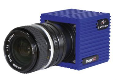
北京欧兰科技发展有限公司为您提供《风洞中速度场,压力场检测方案(CCD相机)》,该方案主要用于航空中速度场,压力场检测,参考标准--,《风洞中速度场,压力场检测方案(CCD相机)》用到的仪器有Imager LX PIV相机、德国LaVision PIV/PLIF粒子成像测速场仪、LaVision DaVis 智能成像软件平台
推荐专场
CCD相机/影像CCD
更多


相关方案
更多
该厂商其他方案
更多