


方案详情
文
LaVision公司的3D3C层析粒子成像测试系统(Tomo-PIV)可以获得瞬时三维体空间流动的全场三分量速度矢量场。利用这一结果数据,通过vortex-in-cell (VIC)方法,可以求出流体压力场。
方案详情

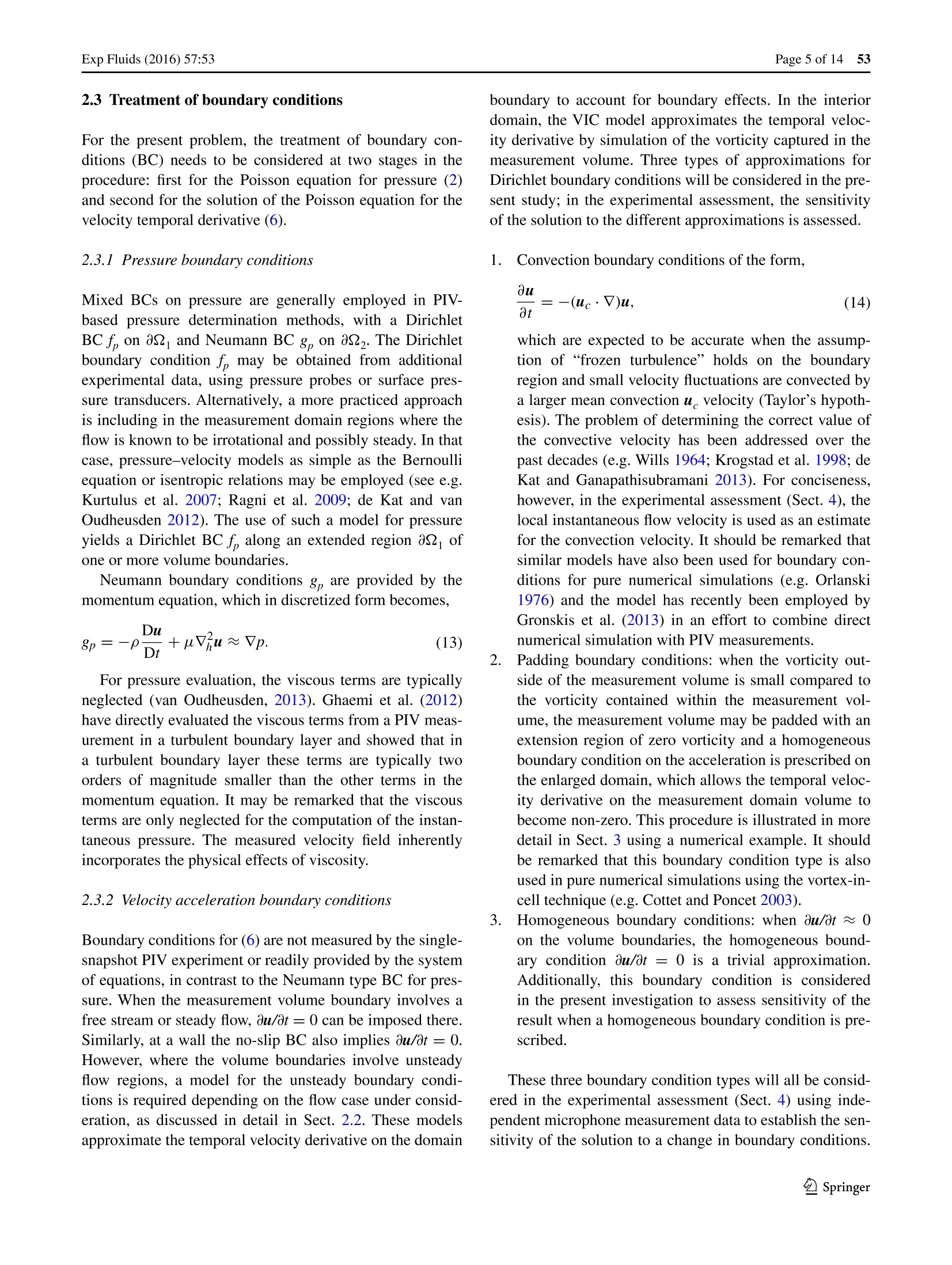
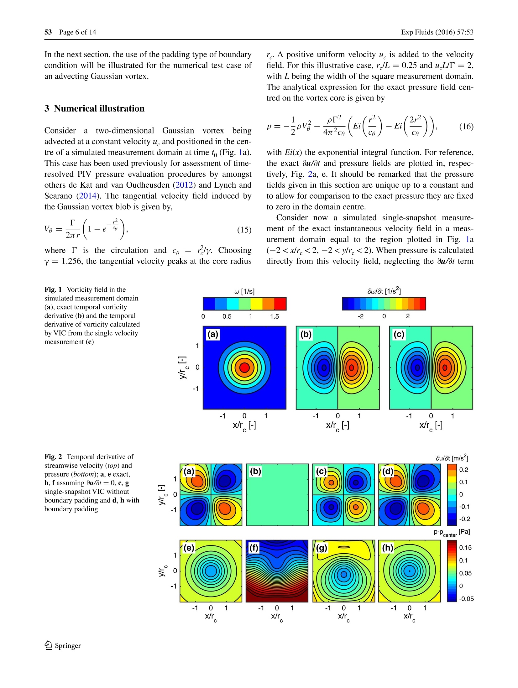
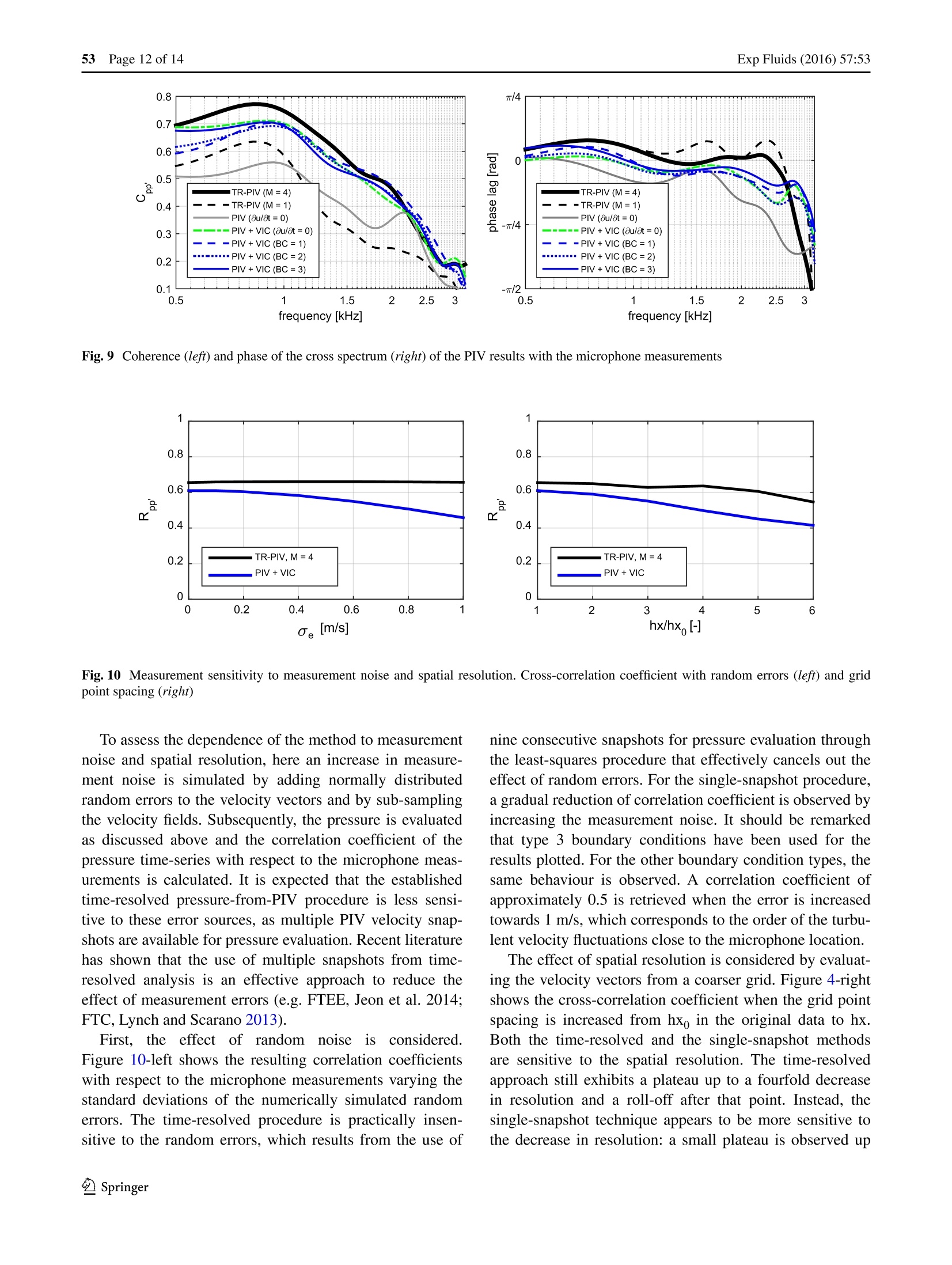
Exp Fluids (2016) 57:53CrossMarkDOI 10.1007/s00348-016-2133-9 Exp Fluids (2016) 57:5353 Page 2 of 14 Pressure estimation from single-snapshot tomographic PIVin a turbulent boundary layer Jan F. G. Schneiders@· Stefan Probsting · Richard P. Dwight· Bas W.van Oudheusden1·Fulvio Scarano Received: 25 January 2015/ Revised: 21 January 2016/ Accepted: 22 January 2016/ Published online: 18 March 2016O The Author(s)2016. This article is published with open access at Springerlink.com Abstract A method is proposed to determine the instanta-neous pressure field from a single tomographic PIV veloc-ity snapshot and is applied to a flat-plate turbulent boundarylayer. The main concept behind the single-snapshot pres-sure evaluation method is to approximate the flow accel-eration using the vorticity transport equation. The vorticityfield calculated from the measured instantaneous velocityis advanced over a single integration time step using thevortex-in-cell (VIC) technique to update the vorticity field,after which the temporal derivative and material derivativeof velocity are evaluated. The pressure in the measurementvolume is subsequently evaluated by solving a Poissonequation. The procedure is validated considering data froma turbulent boundary layer experiment, obtained with time-resolved tomographic PIV at 10 kHz, where an independ-ent surface pressure fluctuation measurement is made bya microphone. The cross-correlation coefficient of the sur-face pressure fluctuations calculated by the single-snapshotpressure method with respect to the microphone measure-ments is calculated and compared to that obtained usingtime-resolved pressure-from-PIV, which is regarded asbenchmark. The single-snapshot procedure returns a cross-correlation comparable to the best result obtained by time-resolved PIV, which uses a nine-point time kernel. Whenthe kernel of the time-resolved approach is reduced to threemeasurements, the single-snapshot method yields approxi-mately 30 % higher correlation. Use of the method shouldbe cautioned when the contributions to fluctuating pressurefrom outside the measurement volume are significant. The ( 区 Ja n F. G. Schneiders ) ( j .f.g.schneiders @tudelft.nl ) Department of Aerospace Engineering, TU Delft,Delft,The Netherlands study illustrates the potential for simplifying the hardwareconfigurations (e.g. high-speed PIV or dual PIV) requiredto determine instantaneous pressure from tomographic PIV. 1 Introduction In only a decade, techniques that determine the fluid flowpressure based on PIV measurements have come to adegree of maturity that justifies their application in practi-cal problems. These developments have been surveyed ina recent review article by van Oudheusden (2013). Startingfrom the work of Liu and Katz (2006), who used a dual-PIV system to measure velocity and its material derivativeand subsequently applied the momentum equation for pres-sure evaluation, all following studies dealing with instan-taneous pressure from PIV have made use of either time-resolved measurements or followed the dual-PIV approach,in order to experimentally determine the velocity materialderivative. It has been shown that an accurate determina-tion of the velocity material derivative in turbulent flowsrequires full three-dimensional evaluation of the veloc-ity and acceleration field, which is currently possible byhigh-speed tomographic PIV experiments (Ghaemi et al.2012). Due to uncorrelated random errors in consecutivePIV snapshots, recent studies have employed a Lagran-gian pseudo-tracking approach to obtain the velocity mate-rial derivative from a series of consecutive time-resolvedvelocity measurements. For example, Liu and Katz (2013)employed five consecutive velocity fields and Novara andScarano (2013) applied a PTV technique to eleven con-secutive camera images. Other studies have focused onnoise reduction of the PIV velocity measurements using forexample a POD-based filtering approach (Charonko et al. 2010) to increase accuracy of the pressure determined fromthe time-resolved PIV measurements. The high sampling rate required for time-resolvedexperiments in airflows compromises the achievable meas-urement volume of tomographic PIV. According to a recentsurvey (Scarano 2013), measurement rates achieved intomo-PIV experiments range from 2.7 kHz (airfoil trail-ing edge by Ghaemi and Scarano 2011; bluff body wakeby de Kat and van Oudheusden 2012) to 5 kHz (turbulentboundary layer by Schroder et al. 2008; rod-airfoil inter-action by Violato et al. 2011). More recent experiments inturbulent boundary layers have been conducted at a rate upto 10 kHz (Ghaemi et al. 2012; Probsting et al.2013), atthe expense of a further reduction of the measurement vol-ume. The above experiments were conducted with airflowvelocities in the range from 7 to 14 m/s, which poses fur-ther restrictions on the value of the Reynolds number. Todate, time-resolved tomographic PIV experiments at flowvelocities on the order of 100 m/s are to be deemed unreal-istic, considering that they would require acquisition rateson the order of 100 kHz. The extension of dual-plane PIV (Kahler and Kompen-hans 2000) or dual-time PIV (Perret et al. 2006) to dual-tomographic PIV systems overcomes the trade-off betweenmeasurement volume and recording rate affecting the time-resolved approach, in that it makes use of two low repeti-tion rate lasers and CCD cameras. Such systems also allowinvestigating flows at higher velocity as one can arbitrarilyreduce the time separation between the two velocity meas-urements, without the restriction set by the repetition rateof a single PIV system. A four-pulse tomographic PIV system has been described (Lynch and Scarano 2014) that canperform acceleration measurements in the compressibleflow regime. The drawback is the complexity associatedwith 8-12 cameras that need to record images from a vol-ume illuminated with two separate dual-pulse lasers. Alternatives to the time-resolvedor dual-PIVapproaches are provided in the field of data assimilation.In periodic flows, phase-locked experiments using non-time-resolved PIV systems have been employed in orderto obtain pressure from a phase-resolved description ofthe flow, as reviewed in van Oudheusden (2013). In addi-tion, not relying on phase-locked experiments, Bai et al.(2015) have employed a reduced-order modelling approachusing compressive sensing for reconstruction of velocitytime-series from PIV measurements performed at limitedtemporal resolution. More advanced methods reconstructboth velocity and pressure by making use of simulation ofthe flow governing equations. Suzuki (2012) proposed areduced-order Kalman filter technique combining PTV andDNS, and later a POD-based hybrid simulation (Suzuki,2014). Recently, Gronskis et al. (2013), Lemke and Ses-terhenn (2013) and Vlasenko et al. (2015) have proposed variational techniques for combination of numerical flowsimulations with PIV measurement results. An advantageof these approaches is that they can naturally incorporatealso local information from other measurement devices(e.g., surface pressure measurements) as alternative or inaddition to PIV. Computational cost associated with thevariational or Kalman-filter-based techniques has, how-ever, limited practical application to real-world volumetricexperiments. Lessccomputationallyy expensivecdata assimilationapproaches solve directly the flow governing equationsusing the PIV data as initial or boundary conditions. Forexample, the use of CFD simulations to fill gaps in themeasurement domain has been discussed by Sciacchitanoet al. (2012). To alleviate measurement rate requirementswhich limit current pressure-from-PIV setups, Scaranoand Moore (2011) proposed to leverage directly the spa-tial information available by the measurement to increasetemporal resolution (“time-supersampling”) using a lin-earized model. The work is based on the assumption offrozen turbulence and advects spatial velocity fluctuationsto produce intermediate velocity estimates in between themeasured samples. The relatively low computational costof the linearized model has allowed for demonstration ofthe method on real-world tomographic PIV data. A simi-lar approach was later used by de Kat and Ganapathisub-ramani (2013), who discussed the importance of estimatingthe local convection velocity. To avoid this, the time-super-sampling concept was generalized to broader flow regimes(separated flows, vortex-dominated regimes) by Schneiderset al. (2014), who introduced the use of the vortex-in-cell(VIC) technique for time-supersampling of tomographicPIV measurements in incompressible flows. The measuredsamples of the velocity field are used both as initial andfinal conditions for a numerical simulation of the vorticitytransport equation, which is solved within the measurementdomain. The study returned an accurate time-reconstruc-tion, demonstrating that the sampling rate requirementscould be significantly reduced with such a procedure. The objective of the present work moves the attention tothe use of VIC on a single velocity field snapshot to esti-mate the instantaneous pressure field in flows where thepressure fluctuations are dominated by vortical structures inthe flow. In particular, the problem of the flat-plate bound-ary layer is considered, which has been studied in recentstudies employing time-resolved tomographic PIV forpressure determination (Ghaemi and Scarano 2011, 2013;Schroder et al. 2011; Probsting et al. 2013, amongst oth-ers). These studies follow two decades of literature on tur-bulent boundary layer flows as reviewed in Marusic et al.(2010). Because of the inherent unsteady nature of theturbulent flow structures in the boundary layer, pressureevaluation from tomographic PIV in such flows has only been demonstrated using a time-resolved (repetition rate~10 kHz) measurement setup. The single-snapshot pressure evaluation using VIC fol-lows a time-marching approach, whereby a single time stepstarting from the instantaneous tomographic PIV velocitymeasurements is needed to approximate the velocity mate-rial derivative and subsequently, the instantaneous pressure.As a result, a significant simplification of the measurementsystems is potentially obtained, with respect to dual sys-tems for the evaluation of pressure-from-PIV. 2 Pressure evaluation from a single PIV velocityfield The discussion here is limited to incompressible and iso-thermal flows. It is furthermore assumed that the velocityfield is measured by tomographic PIV, but the applicationto data from other 3D velocity measurement methods isalso considered possible. Consider a velocity measurementum(x,to) at time t= to on a three-dimensional grid x withconstant spacing h in the volume , which is assumed acuboid with boundary 02. The established time-resolvedpressure-from-PIV procedure solves the Poisson equationfor pressure (van Oudheusden 2013), by approximating “/pr from time-resolved tomographicPIV measurements and with mixed boundary conditionsfand g as detailed in Sect. 2.3.1. The present study alsoemploys (1) for pressure evaluation, but approximates“/pr from a single snapshot. It should be remarked that fordetailed assessment of alternative, established pressure-from-time-resolved-PIV techniques, the reader is referredto Charonko et al. (2010) and van Oudheusden (2013). Inthe present study, second-order central differences are usedin the interior domain and first-order single-sided differ-ences on the domain boundaries. The discretized gradientoperator is denoted by V and the discretized Laplacian byV. The subscript h is used to denote the discretized fieldsand operators. The computational grid is Cartesian andchosen equal to the PIV measurement grid. The discretizedPoisson equation for pressure becomes, The Poisson equation for pressure is discretized usingsecond-order central differences. Ghost points at the exter-nal side of the domain boundary are eliminated through the Neumann boundary condition (see e.g. Ebbers andFarneback 2009). For the unsteady flow regime, time-resolved measure-ments are typically performed to provide "/prlh in theconventional pressure determination approach. Here, it isproposed to approximate the velocity material derivativefrom a single tomographic PIV snapshot by a vortex-in-cell(VIC) simulation (Sect. 2.1). 2.1 Approximation of Du/Dt from single velocitysnapshot From a tomographic PIV velocity measurement um(x,to),vorticity is approximated on the measurement grid, Following the VIC procedure outlined in Schneiderset al. (2014), the divergence-free approximation of themeasured velocity field is calculated by solution of, Although imposing the divergence-free condition hasbeen demonstrated as an effective tool for noise reductionof 3D data (e.g. by de Silva et al. 2013; Schiavazzi et al.2014), in the present study, the divergence-free approxima-tion is an inherent step of the procedure and is not meantfor preconditioning or noise reduction of the measuredvelocity field. In the interior domain, typically uh um,which is mostly ascribed to measurement errors. Recentstudies have proposed to estimate the measurement errorwith the difference between a divergence-free flow fieldand u (Atkinson et al. 2011; Lynch and Scarano 2014;Sciacchitano and Lynch 2015, amongst others). The temporal derivative of vorticity can subsequently becalculated by a finite-difference discretization of the invis-cid vorticity transport equation, The subscript Eul stands here for Eulerian, as later analternative discretization (using VIC) will be introduced.Approximation of 0ω/0t using (5) allows for approxima-tion of the temporal velocity derivative, l, by solution of with Dirichlet boundary conditions fau as discussed inSect. 2.3.2. The velocity material derivative is subsequentlyapproximated by, It should be remarked that solution of(5) requiresapproximation of the gradient of vorticity. VIC avoids thisby employing a vortex particle discretization, as discussedin Schneiders et al. (2014). The VIC time-supersamplingprocedure detailed in the latter paper yields, when appliedto an instantaneous measurement, ω(x,to +At) directlyfrom a single forward-time integration in the interiordomain. Using single-sided finite differences, the temporalvorticity derivative is subsequently approximated, The integration time step is chosen on the order of thePIV pulse time separation; sufficiently small to avoid trun-cation errors, but large enough to avoid rounding errors. Onthetwo grid points adjacent to each volume boundary, theVIC procedure requires boundary values (as discussed irdetail in Schneiders et al. 2014), which are here taken from (5), where i e {1,...,L},j e {1,...,M} and k E {1,...,N} are thegrid points indices in the computational volume. When (9)is employed instead of (5) in the full domain, this improvesthe pressure computation, as reflected by the slight increasein correlation coefficient as witnessed in the experimentalassessment (Sect. 4). 2.2 Range of application and limitations The first limitation regards reconstruction of pressure inflow cases where the pressure associated with the potentialfield dominates pressure associated with the vorticity field.Consider the Helmholtz decomposition of velocity into curlfree and divergence-free parts, u=u+u'. (10c)With this decomposition, Eq. (4) can be rewritten into Thus, the source term of the Poisson equation to recon-struct velocity only contains u’ and therefore the potential field u" is reconstructed using information from the bound-ary points only. As there is typically a much smaller numberof points on the boundary than in the interior, measurementerrors on the domain boundaries are expected to affect umore significantly than u. In flow cases where udominates,sensitivity of the reconstructed potential field to the domainboundary conditions should be cautioned. The present manu-script, however, focusses on a flow case dominated by u. The second limitation follows from the fact that theproposed technique can only use the information avail-able from a single velocity measurement to approximatethe velocity temporal derivative and subsequently pressure.The limitations of the technique become apparent uponsplitting of Eq. (6) into a non-homogeneous Poisson equa-tion with homogeneous boundary conditions and a homo-geneous Poisson equation with non-homogeneous bound-ary conditions, Equation (12a) can be solved directly from the tempo-ral vorticity derivative approximated by (5) from a singletomographic PIV velocity snapshot. However, Eq.(12b)cannot be readily solved in the absence of knowledgeabout the boundary conditions on the temporal velocityderivative, which is not measured by the PIV system. Whenboundary conditions on (12b) cannot be approximated,the pressure field can only be determined up to the pres-sure induced by the irrotational acceleration field follow-ing from Eq. (12b). To illustrate this, consider the extremecase where pressure is determined solely by this compo-nent. Take for example the flow in a cylinder, which is uni-formly accelerated by a piston: a uniform pressure gradi-ent is associated with the acceleration caused by the pistonmotion. As a result, the absolute value of the pressure can-not be determined unless, for this example, the piston pathis known, or in general, when the fluid flow acceleration atthe domain boundary can be estimated. For many relevantapplications in the turbulent flow regime, the instantane-ous value of ou/Ot is dominated by the contribution fromEq. (12a). Such cases include turbulent boundary layers,flow over stationary airfoils, wakes and jets. In additionto the above considerations, in Sect. 2.3.2, three types ofboundary conditions are proposed to approximate boundaryconditions for Eq.(12b) for a wider variety of cases. 2.3 Treatment of boundary conditions For the present problem, the treatment of boundary con-ditions (BC) needs to be considered at two stages in theprocedure: first for the Poisson equation for pressure (2)and second for the solution of the Poisson equation for thevelocity temporal derivative (6). 2.3.1 Pressure boundary conditions Mixed BCs on pressure are generally employed in PIV-based pressure determination methods, with a DirichletBC f, on 09and Neumann BC g, on 02.The Dirichletboundary condition f, may be obtained from additionalexperimental data, using pressure probes or surface pres-sure transducers. Alternatively, a more practiced approachis including in the measurement domain regions where theflow is known to be irrotational and possibly steady. In thatcase, pressure-velocity models as simple as the Bernoulliequation or isentropic relations may be employed (see e.g.Kurtulus et al. 2007; Ragni et al. 2009; de Kat and vanOudheusden 2012). The use of such a model for pressureyields a Dirichlet BC f, along an extended region 02 ofone or more volume boundaries. Neumann boundary conditions g, are provided by themomentum equation, which in discretized form becomes, For pressure evaluation, the viscous terms are typicallyneglected (van Oudheusden, 2013). Ghaemi et al. (2012have directly evaluated the viscous terms from a PIV measurement in a turbulent boundary layer and showed that ina turbulent boundary layer these terms are typically twoorders of magnitude smaller than the other terms in themomentum equation. It may be remarked that the viscousterms are only neglected for the computation of the instan-taneous pressure. The measured velocity field inherentlyincorporates the physical effects of viscosity. 2.3.2 Velocity acceleration boundary conditions Boundary conditions for (6) are not measured by the single-snapshot PIV experiment or readily provided by the systemof equations, in contrast to the Neumann type BC for pres-sure. When the measurement volume boundary involves afree stream or steady flow, ou/0t=0 can be imposed there.Similarly, at a wall the no-slip BC also implies 0u/ot= 0.However, where the volume boundaries involve unsteadyflow regions, a model for the unsteady boundary condi-tions is required depending on the flow case under consid-eration, as discussed in detail in Sect. 2.2. These modelsapproximate the temporal velocity derivative on the domain boundary to account for boundary effects. In the interiordomain, the VIC model approximates the temporal veloc-ity derivative by simulation of the vorticity captured in themeasurement volume. Three types of approximations forDirichlet boundary conditions will be considered in the pre-sent study; in the experimental assessment, the sensitivityof the solution to the different approximations is assessed. 1.Convection boundary conditions of the form, which are expected to be accurate when the assump-tion of “frozen turbulence” holds on the boundaryregion and small velocity fluctuations are convected bya larger mean convection ue velocity (Taylor’s hypoth-esis). The problem of determining the correct value ofthe convective velocity has been addressed over thepast decades (e.g. Wills 1964; Krogstad et al. 1998; deKat and Ganapathisubramani 2013). For conciseness,however, in the experimental assessment (Sect. 4), thelocal instantaneous flow velocity is used as an estimatefor the convection velocity. It should be remarked thatsimilar models have also been used for boundary con-ditions for pure numerical simulations (e.g. Orlanski1976) and the model has recently been employed byGronskis et al. (2013) in an effort to combine directnumerical simulation with PIV measurements. 2. Padding boundary conditions: when the vorticity out-side of the measurement volume is small compared tothe vorticity contained within the measurement vol-ume, the measurement volume may be padded with anextension region of zero vorticity and a homogeneousboundary condition on the acceleration is prescribed onthe enlarged domain, which allows the temporal veloc-ity derivative on the measurement domain volume tobecome non-zero. This procedure is illustrated in moredetail in Sect. 3 using a numerical example. It shouldbe remarked that this boundary condition type is alsoused in pure numerical simulations using the vortex-in-cell technique (e.g. Cottet and Poncet 2003). 3.Homogeneous boundary conditions: when 0u/Ot≈0on the volume boundaries, the homogeneous bound-ary condition ou/Ot = 0 is a trivial approximation.Additionally, this boundary condition is consideredin the present investigation to assess sensitivity of theresult when a homogeneous boundary condition is pre-scribed. These three boundary condition types will all be consid-ered in the experimental assessment (Sect. 4) using inde-pendent microphone measurement data to establish the sen-sitivity of the solution to a change in boundary conditions. In the next section, the use of the padding type of boundarycondition will be illustrated for the numerical test case ofan advecting Gaussian vortex. 3 Numerical illustration Considera two-dimensionalGaussianvortex beingadvected at a constant velocity u and positioned in the cen-tre of a simulated measurement domain at time to(Fig. 1a).This case has been used previously for assessment of time-resolved PIV pressure evaluation procedures by amongstothers de Kat and van Oudheusden (2012) and Lynch andScarano (2014). The tangential velocity field induced bythe Gaussian vortex blob is given by, where I issthe circulation and cg = y. Choosingy= 1.256, the tangential velocity peaks at the core radius r. A positive uniform velocity u is added to the velocityfield. For this illustrative case, r/L=0.25 and u L/T = 2,with L being the width of the square measurement domain.The analytical expression for the exact pressure field cen-tred on the vortex core is given by with Ei(x) the exponential integral function. For reference,the exact Ou/Ot and pressure fields are plotted in, respec-tively, Fig. 2a, e. It should be remarked that the pressurefields given in this section are unique up to a constant andto allow for comparison to the exact pressure they are fixedto zero in the domain centre. Consider nowaa simulated single-snapshot measure-ment of the exact instantaneous velocity field in a meas-urement domain equal to the region plotted in Fig. 1a(-2
确定
还剩12页未读,是否继续阅读?

产品配置单

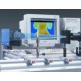
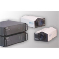
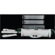
北京欧兰科技发展有限公司为您提供《流体中压力检测方案(粒子图像测速)》,该方案主要用于其他中压力检测,参考标准--,《流体中压力检测方案(粒子图像测速)》用到的仪器有体视层析粒子成像测速系统(Tomo-PIV)、Imager sCMOS PIV相机、PLIF平面激光诱导荧光火焰燃烧检测系统、激光相位多普勒干涉仪LDV,PDI,PDPA,PDA、Artium PDI-FP 双量程可机载飞行探头
相关方案
更多
该厂商其他方案
更多