


方案详情
文
The flow around a ship at yaw angles beyond those
encountered during manoeuvres has not been the
subject of much research reported in the literature.
These conditions are particularly important for an
escort tug, since it uses large yaw angles to generate
hydrodynamic forces that are used to control a ship
(normally a tanker) in the event of an emergency.
This paper presents CFD predictions for the flow
around an escort tug at a yaw angle of 45 degrees and
compares them to PIV measurements of the flow
patterns. The CFD code predicts the essential
features measured within the flow, such as the
separation of the flow from the upstream bilge, and
the formation of a large vortex generated by the low
aspect ratio fin. The predicted vectors were compared
with the measured ones using a numerical technique,
and the agreements were found, on average, to be
within 10%. This level of agreement was within the
estimated uncertainty of the PIV system used for the
experiments.
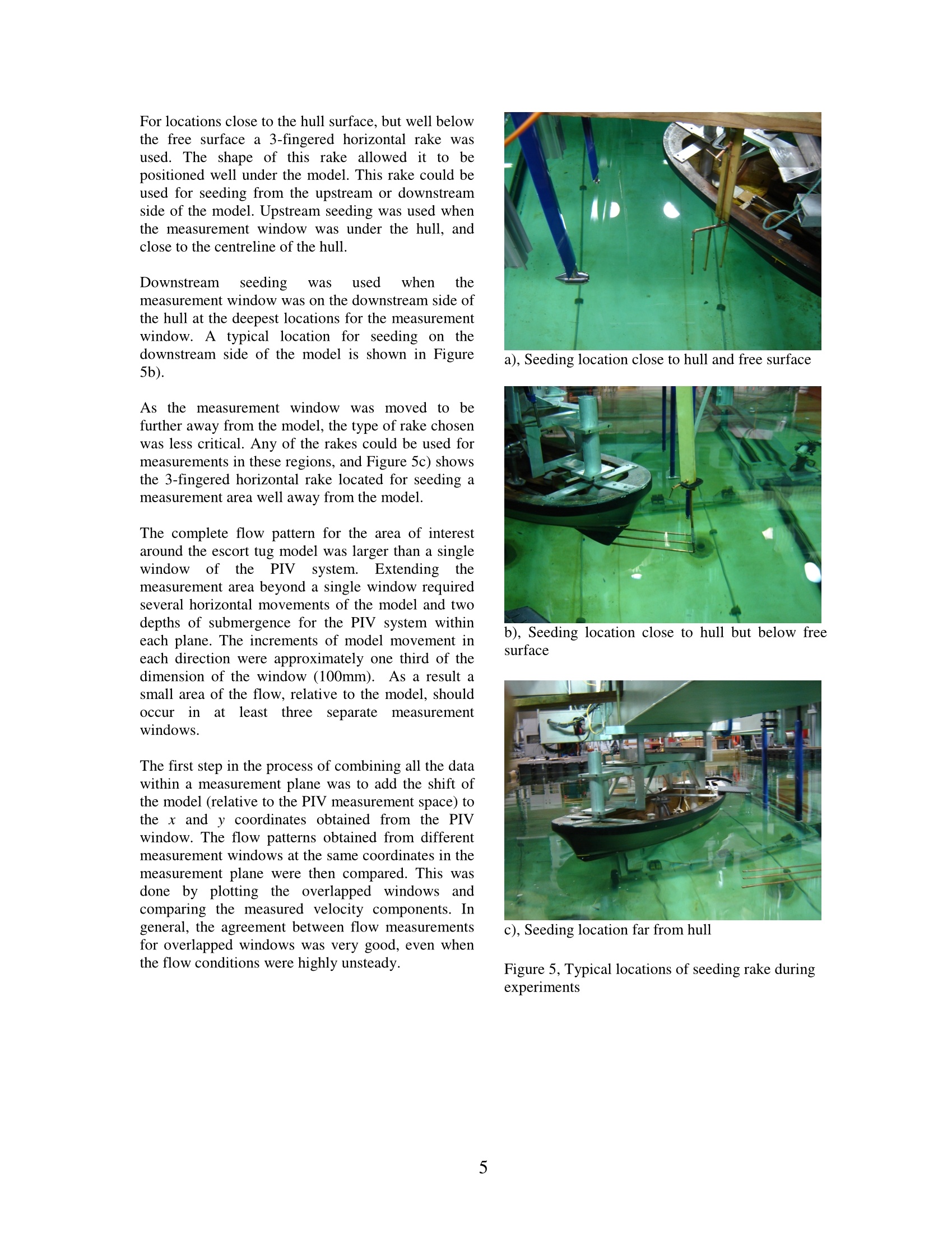
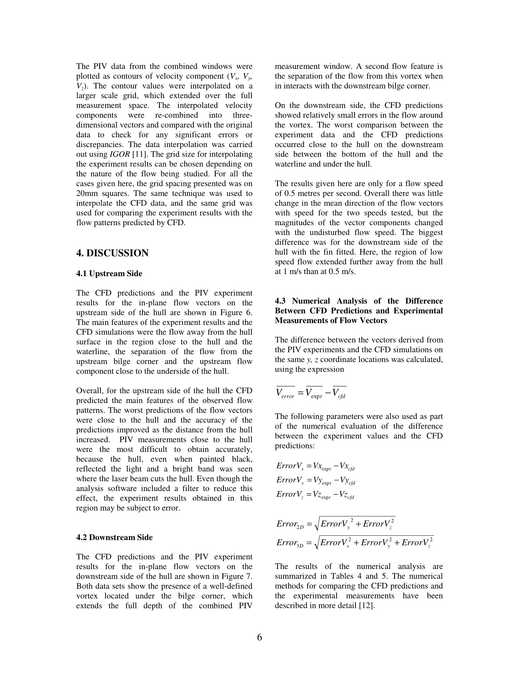
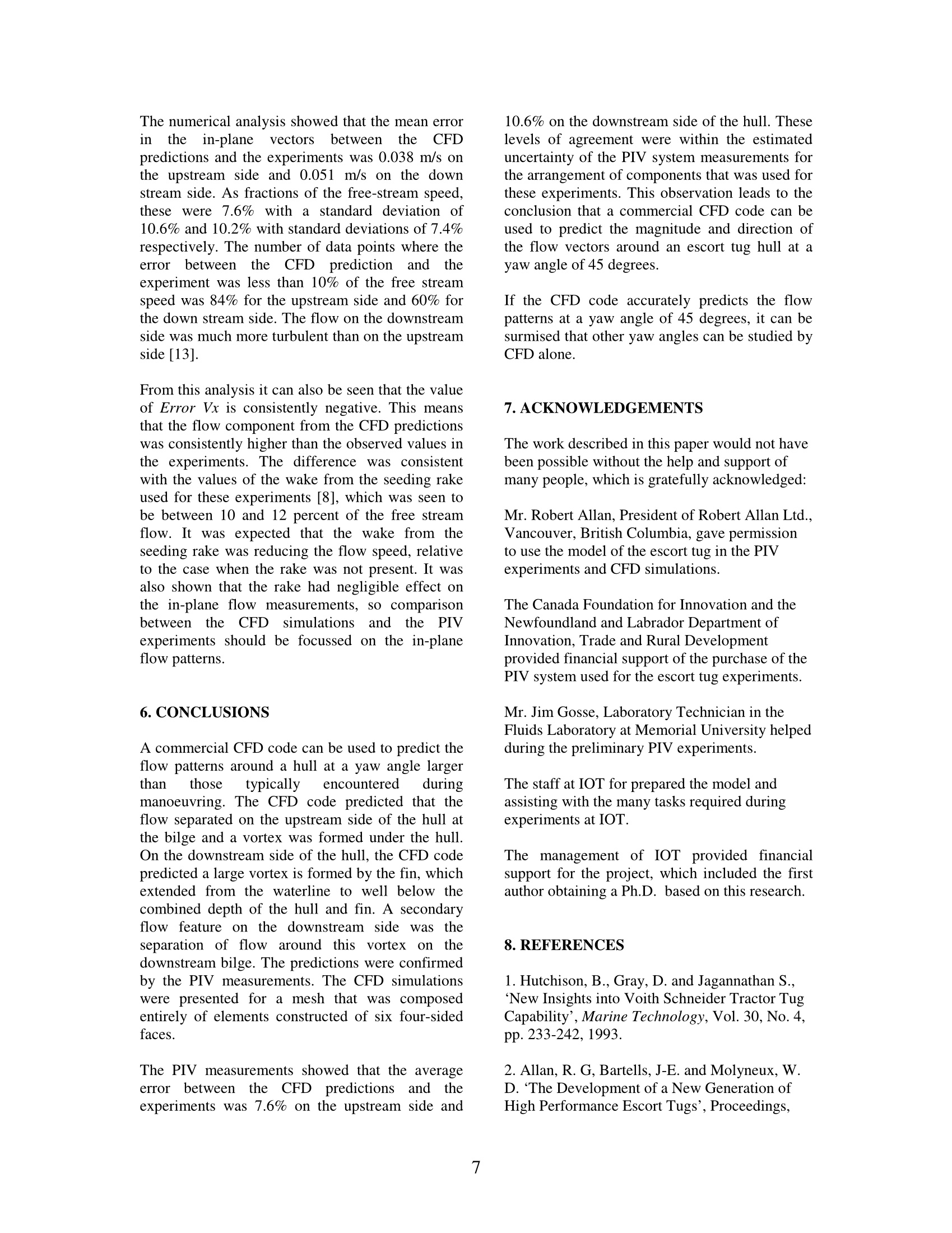
方案详情

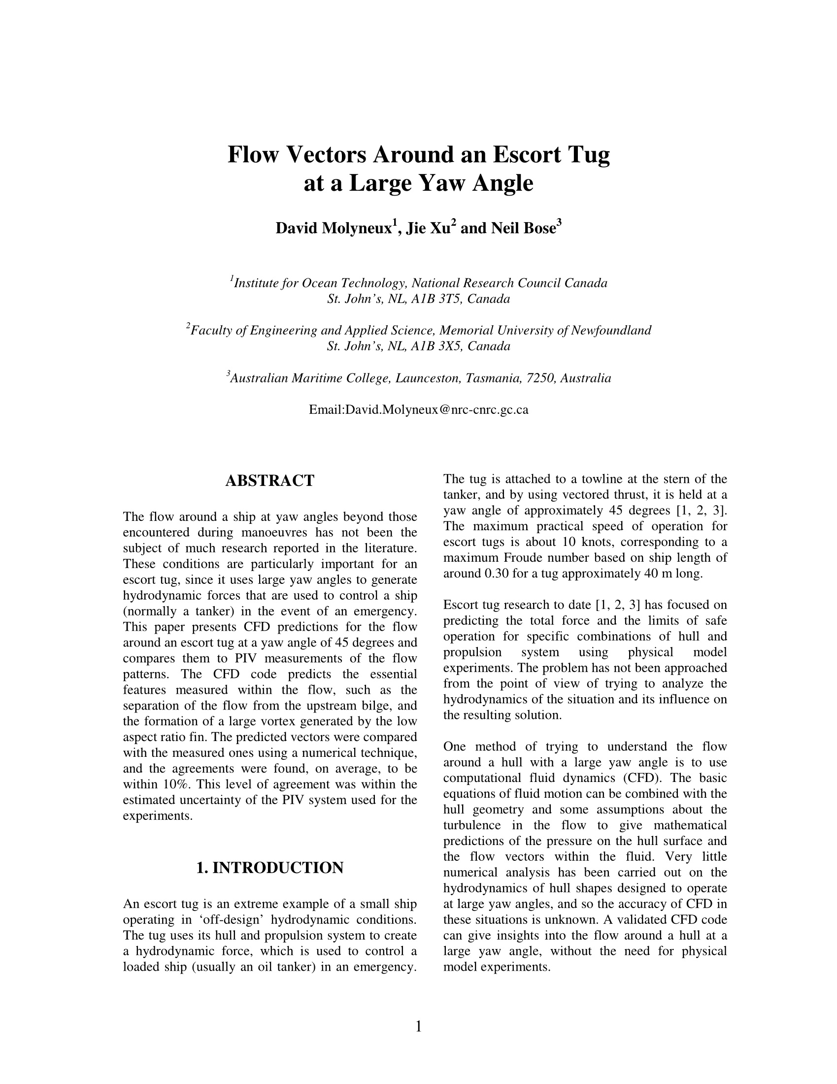
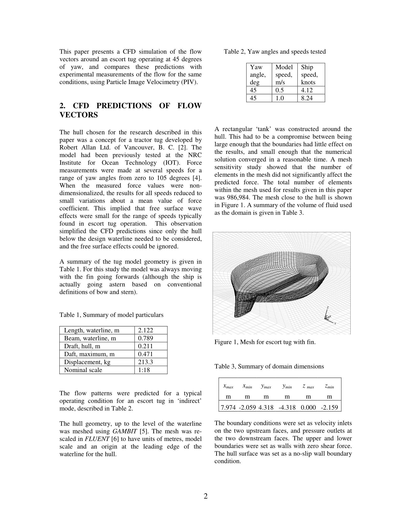
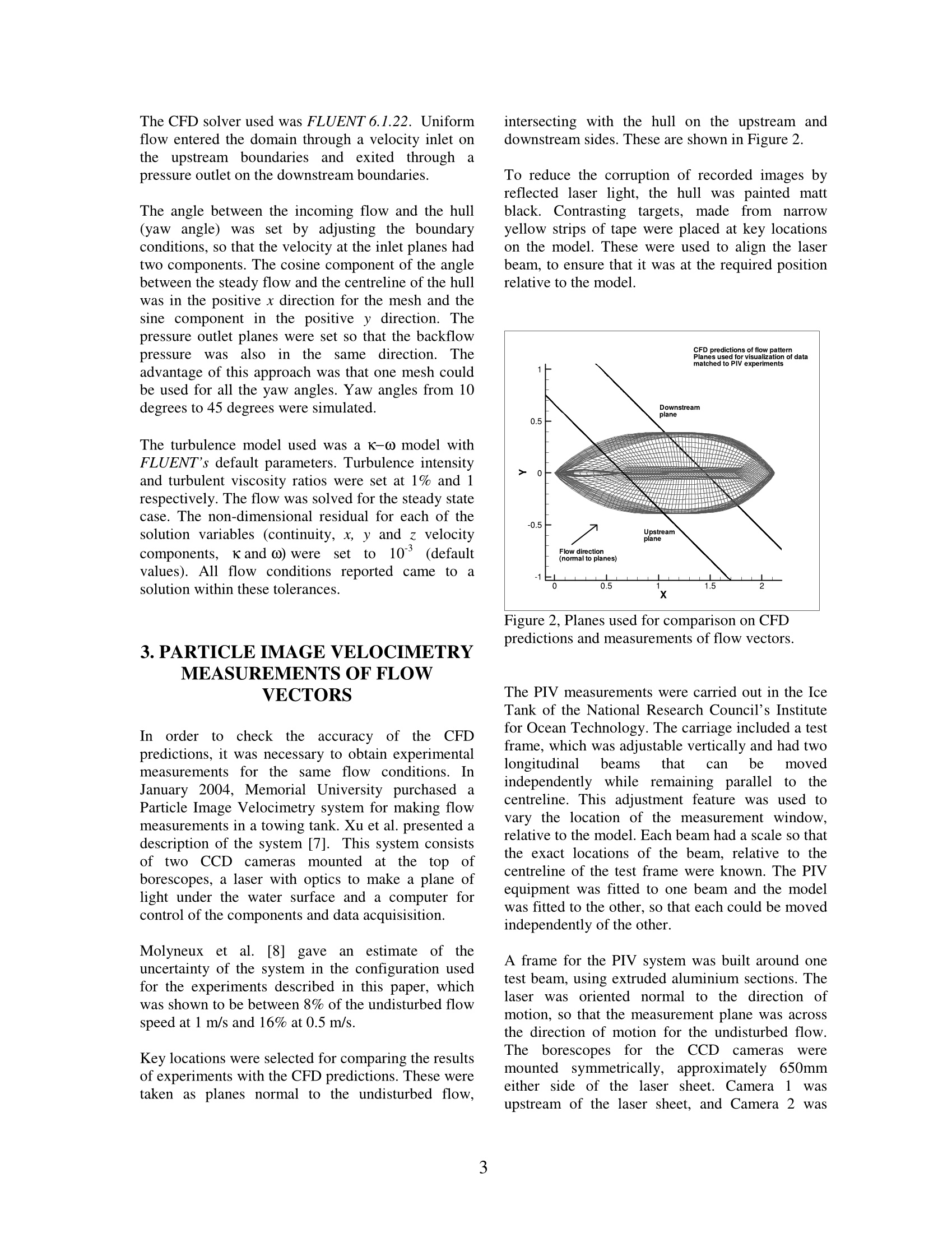
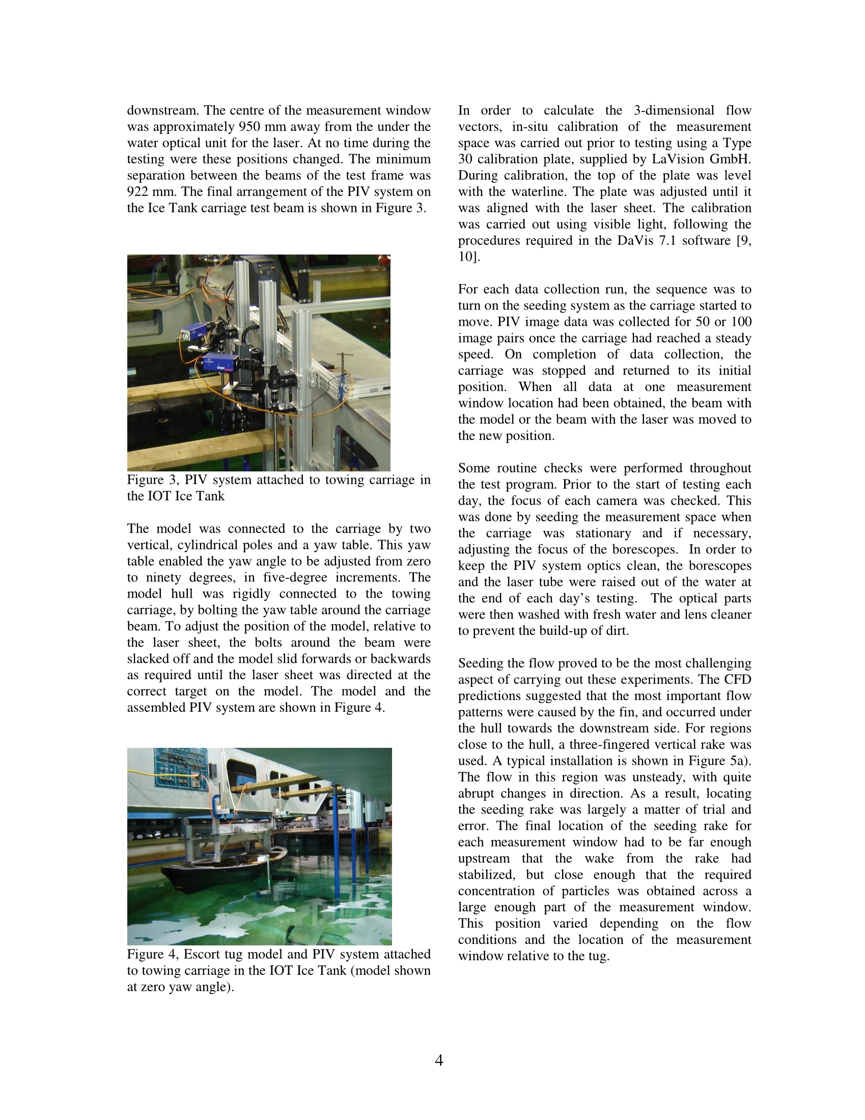
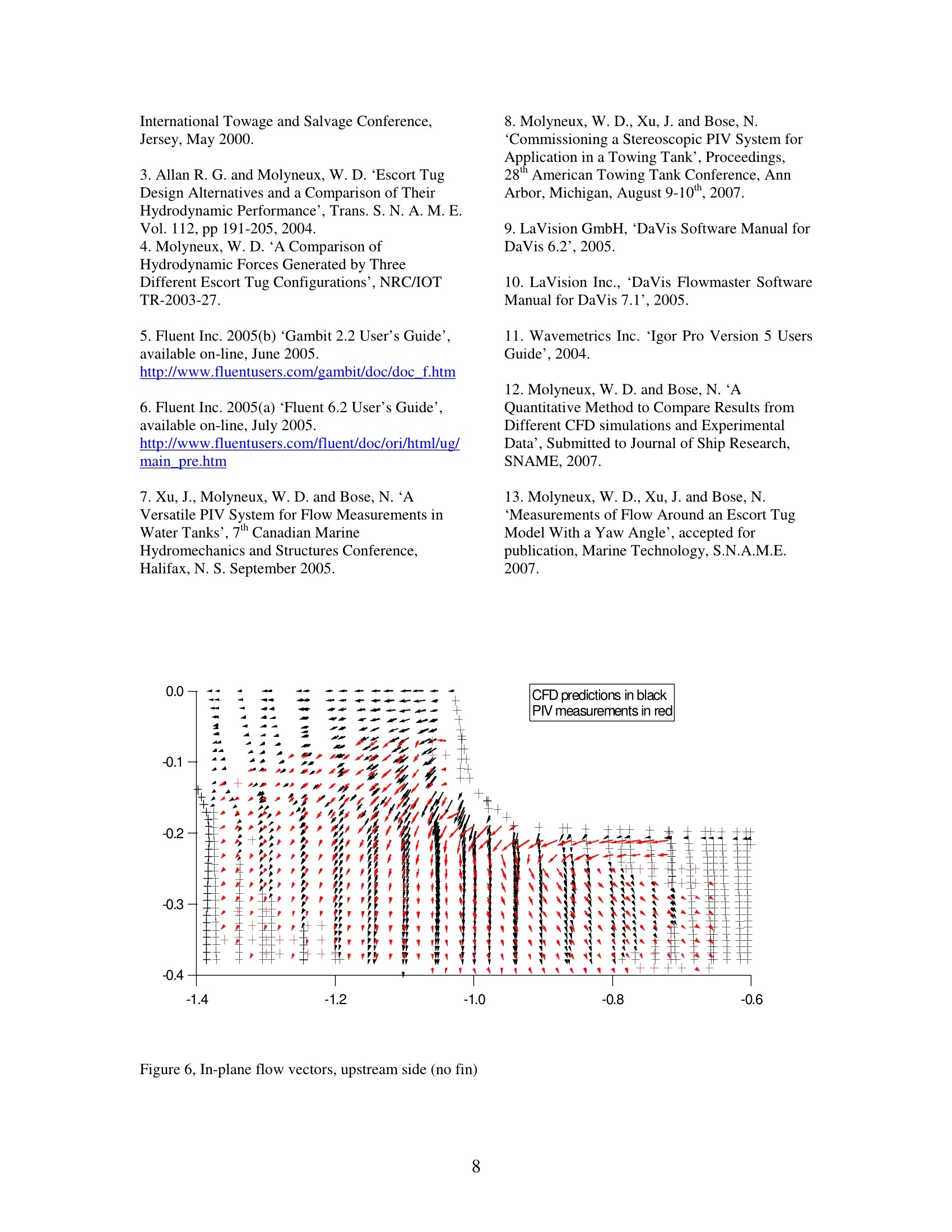
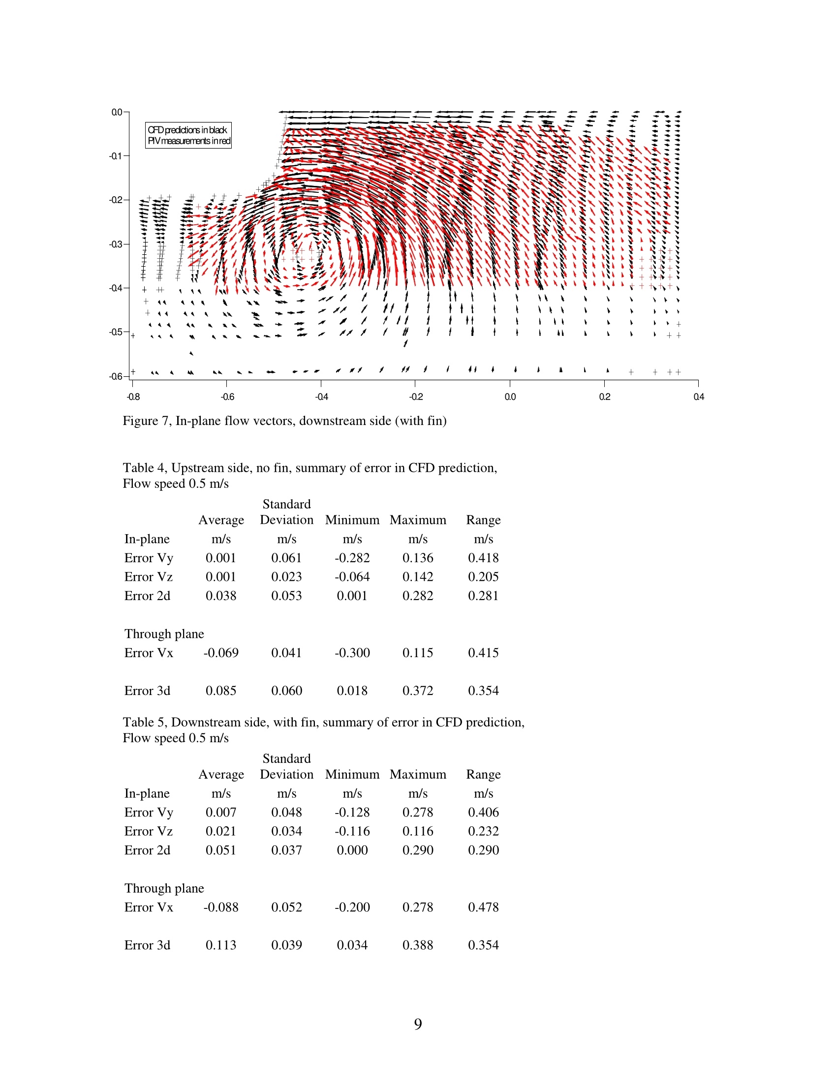
Flow Vectors Around an Escort Tugat a Large Yaw Angle David Molyneux, Jie Xu’ and Neil Bose’ ‘Institute for Ocean Technology, National Research Council CanadaSt. John’s, NL, AlB 3T5, Canada Faculty of Engineering and Applied Science, Memorial University ofNewfoundlandSt. John’s, NL, AIB 3X5, Canada Australian Maritime College, Launceston, Tasmania, 7250, Australia Email:David.Molyneux@nrc-cnrc.gc.ca ABSTRACT The flow around a ship at yaw angles beyond thoseencountered during manoeuvres has not been thesubject of much research reported in the literature.These conditions are particularly important for anescort tug, since it uses large yaw angles to generatehydrodynamic forces that are used to control a ship(normally a tanker) in the event of an emergency.This paper presents CFD predictions for the flowaround an escort tug at a yaw angle of 45 degrees andcompares them to PIV measurements of the flowpatterns.The CFD codepredictsthe essentialfeatures measured within the flow, sucht asistheseparation of the flow from the upstream bilge, andthe formation of a large vortex generated by the lowaspect ratio fin. The predicted vectors were comparedwith the measured ones using a numerical technique,and the agreements were found, on average, to bewithin 10%. This level of agreement was within theestimated uncertainty of the PIV system used for theexperiments. 1.INTRODUCTION An escort tug is an extreme example of a small shipoperating in ‘off-design’hydrodynamic conditions.The tug uses its hull and propulsion system to createa hydrodynamic force, which is used to control aloaded ship (usually an oil tanker) in an emergency. The tug is attached to a towline at the stern of thetanker, and by using vectored thrust, it is held at ayaw angle of approximately 45 degrees [1, 2, 3].The maximum practical speed of operation forescort tugs is about 10 knots, corresponding to amaximum Froude number based on ship length ofaround 0.30 for a tug approximately 40 m long. Escort tug research to date [1, 2, 3] has focused onpredicting the total force and the limits of safeoperation for specific combinations of hull andpropulsion system using physical modelexperiments. The problem has not been approachedfrom the point of view of trying to analyze thehydrodynamics of the situation and its influence onthe resulting solution. One method of trying to understand the flowaround a hull with a large yaw angle is to usecomputational fluid dynamics (CFD). The basicequations of fluid motion can be combined with thehull geometry and some assumptions about theturbulence inittheflowtogive mathematicalpredictions of the pressure on the hull surface andthe flow vectors within the fluid. Very littlenumerical analysis has been carried out on thehydrodynamics of hull shapes designed to operateat large yaw angles, and so the accuracy of CFD inthese situations is unknown. A validated CFD codecan give insights into the flow around a hull at alarge yaw angle, without the need for physicalmodel experiments. This paper presents a CFD simulation of the flowvectors around an escort tug operating at 45 degreesof yaw, and compares these predictions withexperimental measurements of the flow for the sameconditions, using Particle Image Velocimetry (PIV). 2. CFDPREDICTIONSOF ]FLOWVECTORS The hull chosen for the research described in thispaper was a concept for a tractor tug developed byRobert Allan Ltd. of Vancouver, B. C. [2]. Themodel had been previously tested at the NRCInstitute for OceaniTechnology (IOT). Forcemeasurements were made at several speeds for arange of yaw angles from zero to 105 degrees [4].When the measured force values were non-dimensionalized, the results for all speeds reduced tosmall variations about a mean value of forcecoefficient. This implied that free surface waveeffects were small for the range of speeds typicallyfound in escort tug operation.This observationsimplified the CFD predictions since only the hullbelow the design waterline needed to be considered,and the free surface effects could be ignored. A summary of the tug model geometry is given inTable 1. For this study the model was always movingwith the fin going forwards (although the ship isactuallygoing: astern basedonconventionaldefinitions of bow and stern). Table 1, Summary of model particulars Length, waterline, m 2.122 Beam, waterline, m 0.789 Draft, hull, m 0.211 Daft, maximum,m 0.471 Displacement,kg 213.3 Nominal scale 1:18 The flow patterns were predicted for a typicaloperating condition for an escort tug in ‘indirect’mode, described in Table 2. The hull geometry, up to the level of the waterlinewas meshed using GAMBIT [5]. The mesh was re-scaled in FLUENT [6] to have units of metres, modelscale and an origin at the leading edge of thewaterline for the hull. Table 2, Yaw angles and speeds tested Yawangle,deg Modelspeed,m/s Shipspeed,knots 45 0.5 4.12 45 1.0 8.24 A rectangular tank’ was constructed around thehull. This had to be a compromise between beinglarge enough that the boundaries had little effect onthe results, and small enough that the numericalsolution converged in a reasonable time. A meshsensitivity study showed that the number ofelements in the mesh did not significantly affect thepredicted force. The total number of elementswithin the mesh used for results given in this paperwas 986,984. The mesh close to the hull is shownin Figure 1. A summary of the volume of fluid usedas the domain is given in Table3. Figure 1, Mesh for escort tug with fin. Table 3, Summary of domain dimensions Xmax Xmin ymax ymin Z max Zmin m m m m m m 7.974 -2.059 4.318 -4.318 5 0.000 ) -2.159 The boundary conditions were set as velocity inletson the two upstream faces, and pressure outlets atthe two downstream faces. The upper and lowerboundaries were set as walls with zero shear force.The hull surface was set as a no-slip wall boundarycondition. The CFD solver used was FLUENT 6.1.22. Uniformflow entered the domain through a velocity inlet onthe upstream boundariesSiand exitedthroughhapressure outlet on the downstream boundaries. The angle between the incoming flow and the hull(yaw angle) was set by adjusting the boundaryconditions, so that the velocity at the inlet planes hadtwo components. The cosine component of the anglebetween the steady flow and the centreline of the hullwas in the positive x direction for the mesh and thesine component in the positive y direction. Thepressure outlet planes were set so that the backflowpressurewas also in the same direction. Theadvantage of this approach was that one mesh couldbe used for all the yaw angles. Yaw angles from 10degrees to 45 degrees were simulated. The turbulence model used was a K-0 model withFLUENT's default parameters. Turbulence intensityand turbulent viscosity ratios were set at 1% and 1respectively. The flow was solved for the steady statecase. The non-dimensional residual for each of thesolution variables (continuity, x, y and z velocitycomponents,K andω) were setetto10((defaultvalues). All flow conditions reported came to asolution within these tolerances. 3. PARTICLE IMAGE VELOCIMETRYMEASUREMENTS OF FLOWVECTORS lnorder tocheckkthe accuracy of the CFDpredictions, it was necessary to obtain experimentalmeasurements for the same flow conditions. InJanuary 2004, Memorial University purchased aParticle Image Velocimetry system for making flowmeasurements in a towing tank. Xu et al. presented adescription of the system [7]. This system consistsof two CCD camerasmountedatthe top ofborescopes, a laser with optics to make a plane oflight under the water surface and a computer forcontrol of the components and data acquisisition. Molyneux etett all.. [8] ga an estimate of theuncertainty of the system in the configuration usedfor the experiments described in this paper, whichwas shown to be between 8% of the undisturbed flowspeed at 1 m/s and 16% at 0.5 m/s. Key locations were selected for comparing the resultsof experiments with the CFD predictions. These weretaken as planes normal to the undisturbed flow, intersecting with the hull on the upstream anddownstream sides. These are shown in Figure 2. To reduce the corruption of recorded images byreflected laser light, the hull was painted mattblack. Contrasting targets, made from narrowyellow strips of tape were placed at key locationson the model. These were used to align the laserbeam, to ensure that it was at the required positionrelative to the model. Figure 2, Planes used for comparison on CFDpredictions and measurements of flow vectors. The PIV measurements were carried out in the IceTank of the National Research Council’s Institutefor Ocean Technology. The carriage included a testframe, which was adjustable vertically and had twolongitudinal beamsis that canin be movedindependently while remaining parallelto thecentreline. This adjustment feature was used tovary the location of the measurement window,relative to the model. Each beam had a scale so thatthe exact locations of the beam, relative to thecentreline of the test frame were known. The PIVequipment was fitted to one beam and the modelwas fitted to the other, so that each could be movedindependently of the other. A frame for the PIV system was built around onetest beam, using extruded aluminium sections. Thelaser wasoriented normal to the direction ofmotion, so that the measurement plane was acrossthe direction of motion for the undisturbed flow.The borescopes for the CCD cameras weremounted symmetrically, approximately650mmeither side of the laser sheet. Camera 1wasupstream of the laser sheet, and Camera 2was downstream. The centre of the measurement windowwas approximately 950 mm away from the under thewater optical unit for the laser. At no time during thetesting were these positions changed. The minimumseparation between the beams of the test frame was922 mm. The final arrangement of the PIV system onthe Ice Tank carriage test beam is shown in Figure 3. Figure 3, PIV system attached to towing carriage inthe IOT Ice Tank The model was connected to the carriage by twovertical, cylindrical poles and a yaw table. This yawtable enabled the yaw angle to be adjusted from zeroto ninety degrees, in five-degree increments. Themodel hull was rigidly connected to the towingcarriage, by bolting the yaw table around the carriagebeam. To adjust the position of the model, relative tothe laser sheet, the bolts around the beam wereslacked off and the model slid forwards or backwardsas required until the laser sheet was directed at thecorrect target on the model. The model and theassembled PIV system are shown in Figure 4. Figure 4, Escort tug model and PIV system attachedto towing carriage in the IOT Ice Tank (model shownat zero yaw angle). In order to calculate thee3-dimensionalfflowvectors, in-situ calibration of the measurementspace was carried out prior to testing using a Type30 calibration plate, supplied by LaVision GmbH.During calibration, the top of the plate was levelwith the waterline. The plate was adjusted until itwas aligned with the laser sheet. The calibrationwas carried out using visible light, following theprocedures required in the DaVis 7.1 software [9,10]. For each data collection run, the sequence was toturn on the seeding system as the carriage started tomove. PIV image data was collected for 50 or 100image pairs once the carriage had reached a steadyspeed. On completion of data collection, thecarriage was stopped and returned to its initialposition. When all dataattonemeasurementwindow location had been obtained, the beam withthe model or the beam with the laser was moved tothe new position. Some routine checks were performed throughoutthe test program. Prior to the start of testing eachday, the focus of each camera was checked. Thiswas done by seeding the measurement space whenthe carriagewas stationary and if necessary,adjusting the focus of the borescopes. In order tokeep the PIV system optics clean, the borescopesand the laser tube were raised out of the water atthe end of each day’s testing.The optical partswere then washed with fresh water and lens cleanerto prevent the build-upof dirt. Seeding the flow proved to be the most challengingaspect of carrying out these experiments. The CFDpredictions suggested that the most important flowpatterns were caused by the fin, and occurred underthe hull towards the downstream side. For regionsclose to the hull, a three-fingered vertical rake wasused. A typical installation is shown in Figure 5a).The flow in this region was unsteady,with quiteabrupt changes in direction. As a result, locatingthe seeding rake was largely a matter of trial anderror. The final location of the seeding rake foreach measurement window had to be far enoughupstreamntrthattheie ywake from the rakehadstabilized, but close enough that the requiredconcentration of particles was obtained across alarge enough part of the measurement window.Thisspositionvaried dependinggonnthe flowconditions and the location of the measurementwindow relative to the tug. For locations close to the hull surface, but well belowthe free surface a 3-fingered horizontal rake wasused. The shape of this rake allowed it to bepositioned well under the model. This rake could beused for seeding from the upstream or downstreamside of the model. Upstream seeding was used whenthe measurement window was under the hull, andclose to the centreline of the hull. Downstream seeding was used when themeasurement window was on the downstream side ofthe hull at the deepest locations for the measurementwindow. A typical location for seeding on thedownstream side of the model is shown in Figure5b). As the measurement windowwassrmoved to befurther away from the model, the type of rake chosenwas less critical. Any of the rakes could be used formeasurements in these regions, and Figure 5c) showsthe 3-fingered horizontal rake located for seeding ameasurement area well away from the model. The complete flow pattern for the area of interestaround the escort tug model was larger than a singlewindow ofthe pivsystem. Extendingthemeasurement area beyond a single window requiredseveral horizontal movements of the model and twodepths of submergence for the PIV system withineach plane. The increments of model movement ineach direction were approximately one third of thedimension of the window (100mm). As a result asmall area of the flow, relative to the model, shouldOccurir at leastthreee sseparatee mmeasurementwindows. The first step in the process of combining all the datawithin a measurement plane was to add the shift ofthe model (relative to the PIV measurement space) tothe x and y coordinates obtained from the PIVwindow. The flow patterns obtained from differentmeasurement windows at the same coordinates in themeasurement plane were then compared. This wasdonetby plottingthe overlappedwindowsaandcomparing the measured velocity components. Ingeneral, the agreement between flow measurementsfor overlapped windows was very good, even whenthe flow conditions were highly unsteady. a), Seeding location close to hull and free surface b), Seeding location close to hull but below freesurface c), Seeding location far from hull Figure 5, Typical locations of seeding rake duringexperiments The PIV data from the combined windows wereplotted as contours of velocity component (V, V,V). The contour values were interpolated on alarger scale grid, which extended over the fullmeasurementspace. The interpolated velocitycomponents were re-combined into three-dimensional vectors and compared with the originaldataato checkfor any significant errorssordiscrepancies. The data interpolation was carriedout using IGOR [11]. The grid size for interpolatingthe experiment results can be chosen depending onthe nature of the flow being studied. For all thecases given here, the grid spacing presented was on20mm squares. The same technique was used tointerpolate the CFD data, and the same grid wasused for comparing the experiment results with theflow patterns predicted by CFD. 4.DISCUSSION 4.1 Upstream Side The CFD predictions and the PIV experimentresults for the in-plane: fDlowvectors on theupstream side of the hull are shown in Figure 6.The main features of the experiment results and theCFD simulations were the flow away from the hullsurface in the region close to the hull and thewaterline, the separation of the flow from theupstream bilge corner and the upstream flowcomponent close to the underside of the hull. Overall, for the upstream side of the hull the CFDpredicted the main features of the observed flowpatterns. The worst predictions of the flow vectorswere close to the hull and the accuracy of thepredictions improved as the distance from the hullincreased. PIV measurements close to the hullweretthemosttdifficultto obtain1caccurately,becausetthehull, evenwhenpaintedblack.reflected the light and a bright band was seenwhere the laser beam cuts the hull. Even though theanalysis software included a filter to reduce thiseffect, the experiment results obtained in thisregion may be subject to error. 4.2 Downstream Side The CFD predictions and the PIV experimentresults for the in-plane flowvectors on thedownstream side of the hull are shown in Figure 7.Both data sets show the presence of a well-definedvortexlocated under the bilge corner, whichextendsisththe fulldepth of the combinedPIV measurement window. A second flow feature isthe separation of the flow from this vortex whenin interacts with the downstream bilge corner. On the downstream side, the CFD predictionsshowed relatively small errors in the flow aroundthe vortex. The worst comparison between theexperiment(dataandtthe CFD predictionsoccurred close to the hull on the downstreamside between the bottom of the hull and thewaterline and under the hull. The results given here are only for a flow speedof 0.5 metres per second. Overall there was littlechange in the mean direction of the flow vectorswith speed for the two speeds tested, but themagnitudes of the vector components changedwith the undisturbed flow speed. The biggestdifference was for the downstream side of thehull with the fin fitted. Here, the region of lowspeed flow extended further away from the hullat 1 m/s than at 0.5 m/s. 4.33 Numerical Analysiss of the DifferenceBetween CFD Predictions and ExperimentalMeasurements of Flow Vectors The difference between the vectors derived fromthe PIV experiments and the CFD simulations onthe same y, z coordinate locations was calculated,using the expression The following parameters were also used as partof the numerical evaluation of the differencebetween the experiment values and the CFDpredictions: ErrorV.=Vxexpt-VxcfaErrorV=Vyexpt-VycaErrorV=Vzexpr-VzgaErrorp=ErrorV?+ErrorV’Errorsp=ErrorV?+ErrorV?+ErrorV The resultsts oOf theie: numericcaall analysi aresummarized in Tables 4 and 5. The numericalmethods for comparing the CFD predictions andthee experimental measurements have beendescribed in more detail [12]. The numerical analysis showed that the mean errorin theein-plane vectors between theeCFDpredictions and the experiments was 0.038 m/s onthe upstream side and 0.051 m/s on the downstream side. As fractions of the free-stream speed,these were 7.6% with a standard deviation of10.6% and 10.2% with standard deviations of 7.4%respectively. The number of data points where theerrorbetweenthe CFDpredictionandtheexperiment was less than 10% of the free streamspeed was 84% for the upstream side and 60% forthe down stream side. The flow on the downstreamside was much more turbulent than on the upstreamside [13]. From this analysis it can also be seen that the valueof Error Vx is consistently negative. This meansthat the flow component from the CFD predictionswas consistently higher than the observed values inthe experiments. The difference was consistentwith the values of the wake from the seeding rakeused for these experiments [8], which was seen tobe between 10 and 12 percent of the free streamflow. Itt was expected that the wake from theseeding rake was reducing the flow speed, relativeto the case when the rake was not present. It wasalso shown that the rake had negligible effect onthe in-plane flow measurements, so comparisonbetweenthe CFDsimulationsand theePIVexperiments should be focussed on the in-planetlow patterns. 6. CONCLUSIONS A commercial CFD code can be used to predict theflow patterns around a hull at a yaw angle largerthan those typically encountered duringmanoeuvring. The CFD code predicted that theflow separated on the upstream side of the hull atthe bilge and a vortex was formed under the hull.On the downstream side of the hull, the CFD codepredicted a large vortex is formed by the fin, whichextended from the waterline to well below thecombined depth of the hull and fin. A secondaryflow feature on the downstream sidlee wasSptheseparation of flow around this; vortex on thedownstream bilge. The predictions were confirmedby the PIV measurements. The CFD simulationswere presented for a mesh that was composedentirely of elements constructed of six four-sidedfaces. The PIV measurements showed that the averageerror between the CFD predictionsandtheexperiments was 7.6% on the upstream side and 10.6% on the downstream side of the hull. Theselevels of agreement were within the estimateduncertainty of the PIV system measurements forthe arrangement of components that was used forthese experiments. This observation leads to theconclusion that a commercial CFD code can beused to predict the magnitude and direction ofthe flow vectors around an escort tug hull at ayaw angle of 45 degrees. If the CFD code accurately predicts the flowpatterns at a yaw angle of 45 degrees, it can besurmised that other yaw angles can be studied byCFD alone. 7.ACKNOWLEDGEMENTS The work described in this paper would not havebeen possible without the help and support ofmany people, which is gratefully acknowledged: Mr. Robert Allan, President of Robert Allan Ltd.,Vancouver, British Columbia, gave permissionto use the model of the escort tug in the PIVexperiments and CFD simulations. The Canada Foundation for Innovation and theNewfoundland and Labrador Department ofInnovation, Trade and Rural Developmentprovided financial support of the purchase of thePIV system used for the escort tug experiments. Mr. Jim Gosse, Laboratory Technician in theFluids Laboratory at Memorial University helpedduring the preliminary PIV experiments. The staff at IOT for prepared the model andassisting with the many tasks required duringexperiments at IOT. The management of IOT provided financialsupport for the project, which included the firstauthor obtaining a Ph.D. based on this research. 8. REFERENCES 1. Hutchison, B., Gray, D. and Jagannathan S.,New Insights into Voith Schneider Tractor TugCapability', Marine Technology, Vol. 30, No. 4,pp. 233-242,1993. 2. Allan,R. G, Bartells, J-E. and Molyneux, W.D. “The Development of a New Generation ofHigh Performance Escort Tugs’, Proceedings, International Towage and Salvage Conference,Jersey,May 2000. 3. Allan R. G. and Molyneux, W. D. ‘Escort TugDesign Alternatives and a Comparison of TheirHydrodynamic Performance’, Trans. S.N. A. M. E.Vol. 112, pp 191-205,2004. 4. Molyneux, W. D.‘A Comparison ofHydrodynamic Forces Generated by ThreeDifferent Escort Tug Configurations’,NRC/IOTTR-2003-27. 5. Fluent Inc. 2005(b) ‘Gambit 2.2 User’s Guide’,available on-line, June 2005.http://www.fluentusers.com/gambit/doc/doc f.htm 6. Fluent Inc. 2005(a) ‘Fluent 6.2 User’s Guide’,available on-line, July 2005.http://www.fluentusers.com/fluent/doc/ori/html/ug/main pre.htm 7. Xu, J.,Molyneux, W. D. and Bose, N.‘AVersatile PIV System for Flow Measurements inWater Tanks’, 7th Canadian MarineHydromechanics and Structures Conference,Halifax, N. S. September 2005. ( 8. Molyneux, W.D., Xu, J. and Bose, N.Commissioning a Stereoscopic PIV System for. Applicatio n in a Towing Tank', Proceedings, 28" American Towing Tank Conference, Ann Arbor, Michigan, August 9-10", 2007. ) ( 9. LaVision GmbH, ‘ DaVis Software Manual for DaVis 6.2’,2005. ) ( 10. LaVision Inc . , DaVis F lowmaster S o ftware Manual f o r DaVis 7.1', 2005. ) ( 11. Wavemetrics I nc. Igor P ro V ersion 5 U sers Guide’,2004. ) ( 12. Molyneux, W. D. and Bose, N. ‘A Quantitative Method to Compare Results fromDifferent CFD simulations and Experimental Data’, Submitted to Journal of Ship Research, SNAME, 2007. ) ( 13. Molyneux, W. D., Xu, J. and Bose,N. ‘Measurements of Flow Around an Escort T ug Model With a Yaw Angle', accepted forpublication, Marine Technology,S.N.A.M.E2007. ) Figure 7, In-plane flow vectors, downstream side (with fin) Table 4, Upstream side, no fin, summary of error in CFD prediction,Flow speed 0.5 m/s Standard Average Deviation Minimum l Maximum Range In-plane m/s m/s m/s m/s m/s Error Vv 0.001 0.061 -0.282 0.136 0.418 Error Vz 0.001 0.023 -0.064 0.142 0.205 Error 2d 0.038 0.053 0.001 0.282 0.281 Through plane Error Vx -0.069 0.041 -0.300 0.115 0.415 Error 3d 0.085 0.060 0.018 0.372 0.354 Table 5, Downstream side, with fin, summary of error in CFD prediction,Flow speed 0.5 m/s Standard In-plane m/s m/s m/s m/s m/s Error Vy 0.007 0.048 -0.128 0.278 0.406 Error Vz 0.021 0.034 -0.116 0.116 0.232 Error 2d 0.051 0.037 0.000 0.290 0.290 Through plane Error Vx -0.088 0.052 -0.200 0.278 0.478 Error 3d 0.113 0.039 0.034 0.388 0.354
确定
还剩7页未读,是否继续阅读?

产品配置单

北京欧兰科技发展有限公司为您提供《水流体中速度场检测方案(粒子图像测速)》,该方案主要用于船舶中速度场检测,参考标准--,《水流体中速度场检测方案(粒子图像测速)》用到的仪器有德国LaVision PIV/PLIF粒子成像测速场仪、Imager sCMOS PIV相机
相关方案
更多
该厂商其他方案
更多